Introduction
In this article at the end of last year, we mentioned that we performed galaxy shape classification with CNN (VGG16, ResNet). In this article, we will perform galaxy shape classification with a Transformer-based Vison Transformer (ViT).
Sources
As before, the Galaxy10 DECals Dataset from AstroNN will be used as the teacher data.
- Try fine tuning of Vision Transformer model An article explaining classification and fine tuning by Vision Transformer. I used this page as a reference to perform ViT model and fine tuning.
- Pytorch - Transform summary for use with torchvision Data Augmentation was performed to improve generalization performance (to reduce overlearning). Pytorch uses transform to improve generalization performance (to suppress over-training). This is an article explaining the process.
Vision Transformer model
Same as for VGG16 until DataLoader is created.
Preparation
# Training settings
epochs = 30
lr = 3e-5
gamma = 0.7
seed = 42
device = 'cuda' if torch.cuda.is_available() else 'cpu'
import torch
import torch.nn as nn
import torch.nn.functional as F
import torch.optim as optim
from torch.optim.lr_scheduler import StepLR
from linformer import Linformer
from vit_pytorch.efficient import ViT
import timm
Efficient Attention and parameter setting
efficient_transformer = Linformer(
    dim=128,
    seq_len=49+1,  # 7x7 patches + 1 cls-token
    depth=12,
    heads=8,
    k=64
)
# num_classes must be changed.
# If you do 10 classifications without changing it, you will get the following error.
# The error occurs at the timing of to(device), but there is no cause there.
# RuntimeError: CUDA error: device-side assert triggered
# CUDA kernel errors might be asynchronously reported at some other API call,so the stacktrace below might be incorrect.
# For debugging consider passing CUDA_LAUNCH_BLOCKING=1.
model = ViT(
    dim=128,
    image_size=224,
    patch_size=32,
    num_classes=10,
    transformer=efficient_transformer,
    channels=3,
).to(device)
Configure Ross functions and Optimizer.
# loss function
criterion = nn.CrossEntropyLoss()
# optimizer
optimizer = optim.Adam(model.parameters(), lr=lr)
# scheduler
scheduler = StepLR(optimizer, step_size=1, gamma=gamma)
Training
The training part is basically the same as in the case of VGG16, but we also calculated ACCURACY.
accuracy calculation function
def cal_acc(outputs, labels):
    p_arg = torch.argmax(outputs, dim = 1)
    return torch.sum(labels == p_arg)
Note that the return value of this function is torch.Tensor.
Learning Function
Changed to also return train_acc (the accuracy of the training data at a given epoch).
def train_epoch(model, optimizer, criterion, dataloader, device):
    train_loss = 0
    train_acc = 0
    model.train()
    for i, (images, labels) in enumerate(dataloader):
        images, labels = images.to(device), labels.to(device)
        optimizer.zero_grad()
        outputs = model(images)
        loss = criterion(outputs, labels)
        loss.backward()
        optimizer.step()
        train_loss += loss.item()
        train_acc += cal_acc(outputs, labels).item()
    train_loss = train_loss / len(dataloader.dataset)
    train_acc = train_acc / len(dataloader.dataset)

    return train_loss, train_acc
Inference Function
Changed to also return test_acc (accuracy of test data at a certain epoch).
def inference(model, optimizer, criterion, dataloader, device):
    model.eval()
    test_loss=0
    test_acc = 0

    with torch.no_grad():
        for i, (images, labels) in enumerate(dataloader):
            images, labels = images.to(device), labels.to(device)
            outputs = model(images)
            loss = criterion(outputs, labels)
            test_loss += loss.item()
            test_acc += cal_acc(outputs, labels).item()
        test_loss = test_loss / len(dataloader.dataset)
        test_acc = test_acc / len(dataloader.dataset)
    return test_loss, test_acc
Function to execute a given epoch
Changed to return a list of “accuracy” and “loss” by training/test data.
def run(num_epochs, optimizer, criterion, device):
    train_loss_list = []
    test_loss_list = []
    train_acc_list = []
    test_acc_list = []
    for epoch in range(num_epochs):
        train_loss, train_acc = train_epoch(model, optimizer, criterion, train_loader, device)
        test_loss, test_acc = inference(model, optimizer, criterion, test_loader, device)

        print(f'Epoch [{epoch+1}], train_Loss : {train_loss:.4f}, test_Loss : {test_loss:.4f}, train_acc : {train_acc:.4f}, test_acc : {test_acc:.4f}')
        train_loss_list.append(train_loss)
        test_loss_list.append(test_loss)
        train_acc_list.append(train_acc)
        test_acc_list.append(test_acc)
    return train_loss_list, test_loss_list, train_acc_list, test_acc_list
calling portion
# 訓練時間を測定:開始

import time
import datetime

dt_now = datetime.datetime.now()
print("*** Started the Timer at {} ***".format(dt_now))
start_time = time.time()  # 実行時間計測開始
train_loss_list, test_loss_list, train_acc_list, test_acc_list = run(epochs, optimizer, criterion, device)
# 訓練時間測定:終了

lapse_time = time.time() - start_time
print("-" * 80)
print("実行時間 {:8.1f}秒".format(lapse_time))
print("-" * 80)
dt_now = datetime.datetime.now()
print("*** Stopped the Timer at {} ***".format(dt_now))
Display of accuracy and loss graphs
import matplotlib.pyplot as plt

# Plot loss & accuracy
num_epochs=30

fig = plt.figure(figsize=(12,6), dpi=100)
ax1 = fig.add_subplot(1, 2, 2)  # error in right side
ax2 = fig.add_subplot(1, 2, 1)

ax1.plot(range(num_epochs), train_loss_list, c='b', label='train loss')
ax1.plot(range(num_epochs), test_loss_list, c='r', label='test loss')
ax1.set_xlabel('epoch', fontsize='14')
ax1.set_ylabel('loss', fontsize='14')
ax1.set_title('training and test loss', fontsize='18')
ax1.grid()
ax1.legend(fontsize='18')

ax2.plot(range(num_epochs), train_acc_list, c='b', label='train accuracy')
ax2.plot(range(num_epochs), test_acc_list, c='r', label='test accuracy')
ax2.set_xlabel('epoch', fontsize='14')
ax2.set_ylabel('accuracy', fontsize='14')
ax2.set_title('training and test accuracy', fontsize='18')
ax2.grid()
ax2.legend(fontsize='18')

plt.show()
Execution results
The graph of the execution result is as follows.
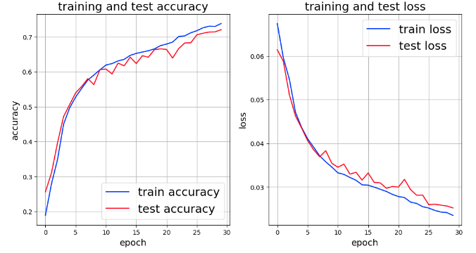
If the Epoch is extended, it seems to improve somewhat, but both accuracy and loss seem to be lower than those of ResNet.
In this article, only loss was graphed, so for reference, so for comparison with ViT’s results, accuracy was also obtained for ResNet. The following graph shows the result.
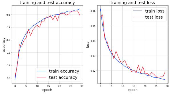
In next time, we will do fine tuning using models that have already been trained.
Translated with www.DeepL.com/Translator (free version)