Speed-up Learning and inference on Pytorch

Motivation

In my home environment where I use NFS to store JupyterLab notebooks, I measured the performance when the NFS server is a RaspberryPi or HP Z240, and found that in the learning loop (state in which epochs are stacked), there is no significant difference whether the NB is stored on an NFS server or locally. I found that there was no significant difference between NBs stored on an NFS server or locally.

Therefore, I have challenged to speed up the learning process, and I summarize the progress/results here.

Information Sources

PyTorchでの学習・推論を高速化するコツ集 I tried three of them in this article.

Environment

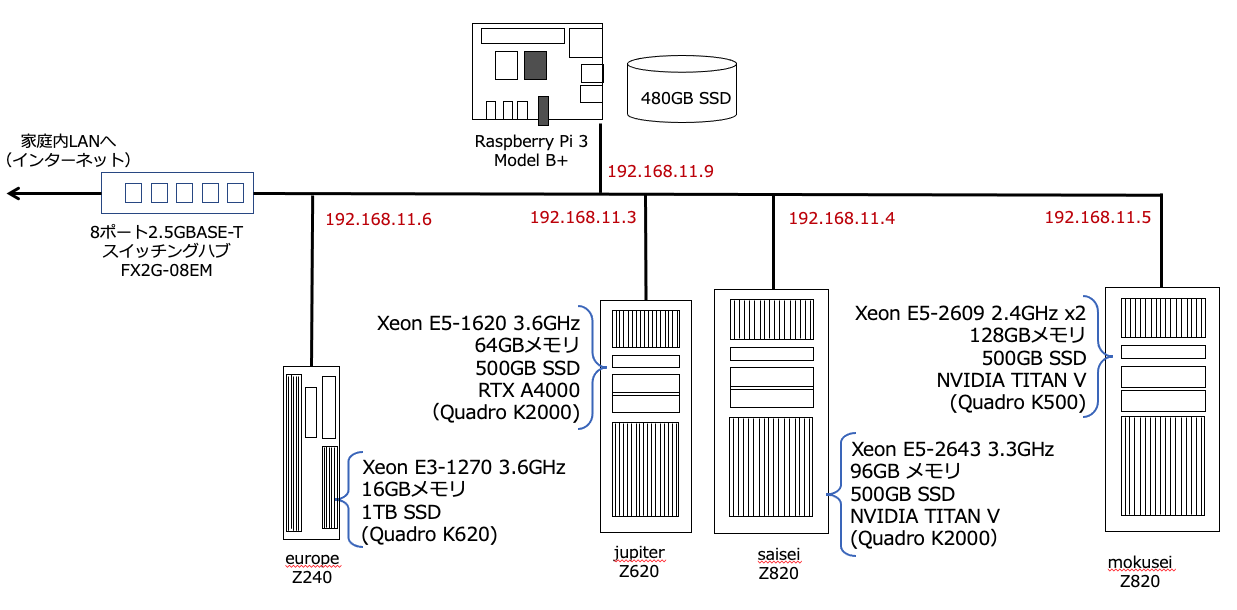
In the following system configuration diagram, JupyterLab is running on saisei and the NoteBooks stored on europe are NFS mounted.

SystemConfigChart

The original program before the speed-up was a program for galaxy shape classification using the vgg16 model presented in this article. The learning rate was set at $lr=0.00001$.

Efforts to increase speed

num_workers

Added “num_workers=2” parameter when creating DataLoader.

# DataLoaderを作成
batch_size = 32
train_loader = DataLoader(train_dataset, batch_size=batch_size, shuffle=True, num_workers=2)
valid_loader = DataLoader(valid_dataset, batch_size=batch_size, shuffle=True, num_workers=2)

pin_memory

Also, add “pin_memory=True” to the parameter for creating DataLoader.

# DataLoaderを作成
batch_size = 32
train_loader = DataLoader(train_dataset, batch_size=batch_size, shuffle=True, num_workers=2, pin_memory=True)
valid_loader = DataLoader(valid_dataset, batch_size=batch_size, shuffle=True, num_workers=2, pin_memory=True)

Introducing AMP (Automatic Mixed Precision)

In the learning and inference loop (1epoch loop), AMP was used and modified as follows.

Learning loop

def train_epoch(model, optimizer, criterion, dataloader, device):
    train_loss = 0
    train_acc = 0
    model.train()
    scaler = torch.cuda.amp.GradScaler()  # add for amp
    for i, (images, labels) in enumerate(dataloader):
        images, labels = images.to(device), labels.to(device)
        optimizer.zero_grad()
        with torch.cuda.amp.autocast():  # add for amp
            outputs = model(images)
            loss = criterion(outputs, labels)
        scaler.scale(loss).backward()  # add for amp
        scaler.step(optimizer)  # add for amp
        scaler.update()  # add for amp
#        loss.backward()
#        optimizer.step()
        train_loss += loss.item()
        train_acc += cal_acc(outputs, labels).item()
    train_loss = train_loss / len(dataloader.dataset)
    train_acc = train_acc / len(dataloader.dataset)
    
    return train_loss, train_acc

Inference loop

def inference(model, optimizer, criterion, dataloader, device):
    model.eval()
    valid_loss=0
    valid_acc = 0
    scaler = torch.cuda.amp.GradScaler()  # add for amp

    with torch.no_grad():
        for i, (images, labels) in enumerate(dataloader):
            images, labels = images.to(device), labels.to(device)
            with torch.cuda.amp.autocast():  # add for amp
                outputs = model(images)
                loss = criterion(outputs, labels)
            valid_loss += loss.item()
            valid_acc += cal_acc(outputs, labels).item()
        valid_loss = valid_loss / len(dataloader.dataset)
        valid_acc = valid_acc / len(dataloader.dataset)
    return valid_loss, valid_acc

Result

The following table shows the results of the run on jupiter (GPU: RTX A4000).

Change factor (cumulative)	Execution time (sec)	Run-time ratio
original	3,342	1.0
＋num_worker	3,198	0.96
＋num_worker＋pin_memory	3,073	0.92
＋num_worker＋pin_memory＋AMP	2,163	0.65

AMP (Automatic Mixed Precision) is a very effective result.

The results of the same conditions, run on saisei (GPU: TITAN V), are as follows.

Change factor (cumulative)	Execution time (sec)	Run-time ratio
オリジナル	2,670	1.0
＋num_worker	2,440	0.91
＋num_worker＋pin_memory	2,339	0.88
＋num_worker＋pin_memory＋AMP	1,558	0.58

Likewise, AMP is highly effective.

From now on, I will use the above three faster versions as standard.