Try Athena++, a magnetohydrodynamic simulation code for astrophysics

Introduction

I have been interested in trying out astrophysics-related simulations for some time, and had been checking out ENZO, GADGET, GIZMO, and others. I happened to know Athena, and when I looked into it, I found that Associate Professor Kengo Tomita of Tohoku University maintains a Japanese page and has some information in Japanese, so I decided to give it a try.

Here, I summarize the process of installing and running the tutorial, and post it.

Sources

Athena++ The original page.
Athena++ Japanese Support Page Japanese page maintained by Mr. Tomita. It is very helpful because it is in Japanese.
Running C++ Numerical Simulations in Docker An article about running Athena++ in a docker container environment.
Tutorial Tutorial to learn after installation, also available from the above sources.

Policy

Athena++ will be installed as a docker container to run the tutorials. First, I will install the minimum amount of software necessary to run the first tutorial in a container. I will build the software into the container as needed. For example, I will build MPI and other software into the docker container in case I want to try it on multiple nodes in the future.

Installation

First Dockerfile

# Based on the Dockefile for creating a Docker image that JupyterLab can use, 
# Create a Docker container that can be used for athena++ development and execution.

# Based on the latest version of ubuntu 22.04.
FROM ubuntu:jammy-20240111

# Set bash as the default shell
ENV SHELL=/bin/bash

# Build with some basic utilities
RUN apt update && apt install -y \
    build-essential \
    python3-pip apt-utils vim \
    git git-lfs \
    curl unzip wget gnuplot

# alias python='python3'
RUN ln -s /usr/bin/python3 /usr/bin/python

# install python package to need
RUN pip install -U pip setuptools \
        && pip install numpy scipy h5py mpmath

# Create a working directory
WORKDIR /workdir

# command prompt
CMD ["/bin/bash"]

Launch Docker

Create and launch a container image from the Dockerfile shown in the previous section.

On the host machine, I decided to download from the public Athena++ Github repository and set the area to /ext/nfs/athena++.

$ cd /ext/nfs/athena++
$ git clone https://github.com/PrincetonUniversity/athena

Run a regression test

Source 1. uses Quick -Start’s Testing that the code runs, and Source 2. uses Athena++ Quick-Start’s method for now. The following is the method of Source 2.

The following is the operation in the docker container that was started.

# pwd
/workdir/athena/tst/regression

# python run_tests.py
・・・
Setup complete, entering main loop...
・・・

Actually, I ran the regression test above and got some errors, so I added the necessary python packages. The aforementioned Dockerfile reflects that.

Run the tutorial

Run 1D Shock Tube

The following is the operation in the docker container that was started.

Go to the given directory

# pwd
/workdir/athena

Setup (create a Makefile)

# python configure.py --prob shock_tube
  Your Athena++ distribution has now been configured with the following options:
  Problem generator:            shock_tube
  Coordinate system:            cartesian
  Equation of state:            adiabatic
  Riemann solver:               hllc
  Magnetic fields:              OFF
  Number of scalars:            0
  Number of chemical species:   0
  Special relativity:           OFF
  General relativity:           OFF
  Radiative Transfer:           OFF
    Implicit Radiation:           OFF
  Cosmic Ray Transport:         OFF
  Frame transformations:        OFF
  Self-Gravity:                 OFF
  Super-Time-Stepping:          OFF
  Chemistry:                    OFF
  KIDA rates:                   OFF
  ChemRadiation:                OFF
  chem_ode_solver:              OFF
  Debug flags:                  OFF
  Code coverage flags:          OFF
  Linker flags:
  Floating-point precision:     double
  Number of ghost cells:        2
  MPI parallelism:              OFF
  OpenMP parallelism:           OFF
  FFT:                          OFF
  HDF5 output:                  OFF
  Compiler:                     g++
  Compilation command:          g++  -O3 -std=c++11

Compile

# make clean

# make

The above will create a.out named athena under the bin directory.

The following is an operation in a working directory in a docker container. In the following example, /workdir/kenji is the working directory.

# pwd
/workdir/kenji

# cp /workdir/athena/inputs/hydro/athinput.sod .
# /workdir/athena/bin/athena -i athinput.sod

Setup complete, entering main loop...

cycle=0 time=0.0000000000000000e+00 dt=2.6411070460266146e-03
cycle=1 time=2.6411070460266146e-03 dt=1.5116606032023513e-03
・・・
cycle=175 time=2.5000000000000000e-01 dt=1.4248899766177968e-03

Terminating on time limit
time=2.5000000000000000e-01 cycle=175
tlim=2.5000000000000000e-01 nlim=-1

zone-cycles = 44800
cpu time used  = 5.6783000000000000e-02
zone-cycles/cpu_second = 7.8896852931335079e+05

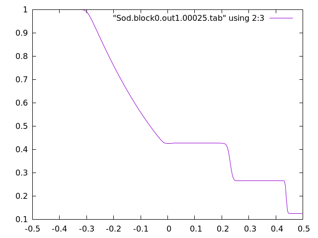
Visualization with gnuplot

# gnuplot

gnuplot> set terminal pngcairo
gnuplot> plot "Sod.block0.out1.00025.tab" using 2:3 with lines
gnuplot> set out "xxx.png"
gnuplot> replot

The xxx.png obtained above is as follows

gnuplot

Visualization with matplotlib

I also performed visualizing using the “Data Visualization” code from source 3.

If you specify the directory of the jupyterlab docker container’s notebook created in this post to be the /workdir directory of the Athena++ docker container with -v, you can display it with matplotlib as follows. workdir directory of the docker container for Athena++ with -v, it can be displayed with matplotlib as follows.

import matplotlib.pyplot as plt
import pandas as pd

# Density

fig, ((ax1, ax2), (ax3, ax4)) = plt.subplots(nrows=2, ncols=2, figsize=(10, 8))
df = pd.read_fwf('Sod.block0.out1.00000.tab',skiprows=1)
ax1.plot(df.x1v, df.rho, 'b', linewidth = 3); ax1.set_title('t=0') 
ax1.set_ylabel('Density', fontsize=12)
df = pd.read_fwf('Sod.block0.out1.00008.tab',skiprows=1)
ax2.plot(df.x1v, df.rho, 'b', linewidth = 3); ax2.set_title('t=8')
ax2.set_ylabel('Density', fontsize=12)
df = pd.read_fwf('Sod.block0.out1.00016.tab',skiprows=1)
ax3.plot(df.x1v, df.rho, 'b', linewidth = 3); ax3.set_title('t=16')
ax3.set_xlabel('shock tube', fontsize=12); ax3.set_ylabel('Density', fontsize=12)
df = pd.read_fwf('Sod.block0.out1.00024.tab',skiprows=1)
ax4.plot(df.x1v, df.rho, 'b', linewidth = 3); ax4.set_title('t=24')
ax4.set_xlabel('shock tube', fontsize=12); ax4.set_ylabel('Density', fontsize=12)
plt.show()

matplotlib

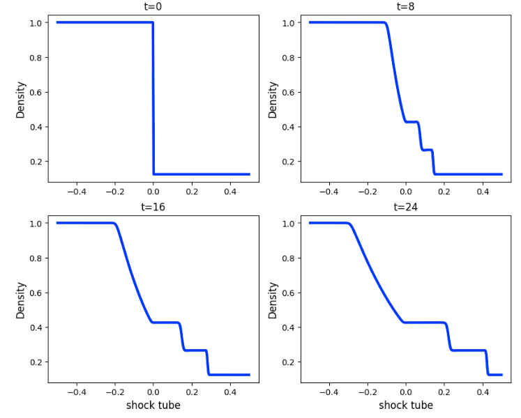
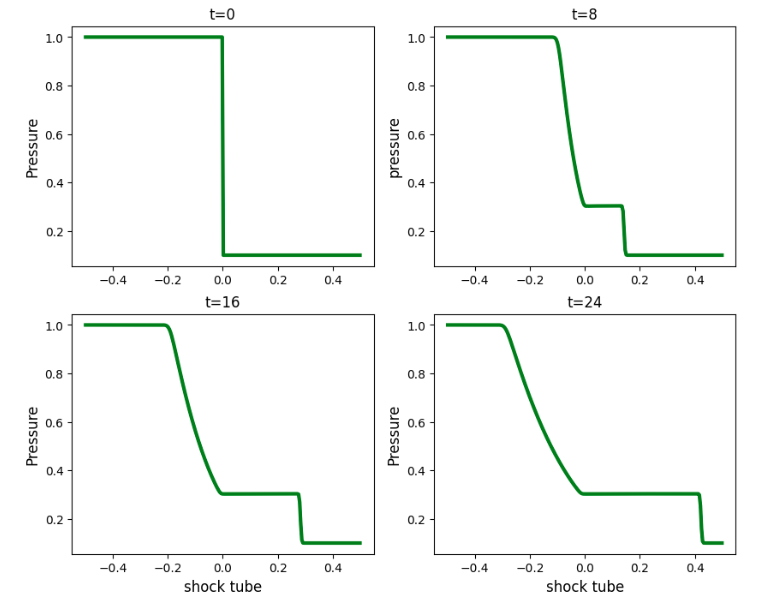
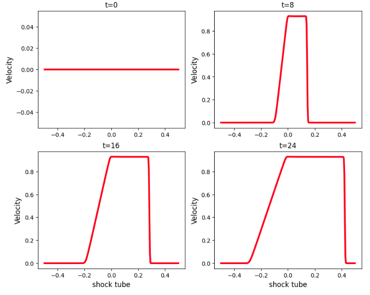
By changing each string in the above code as shown in the table below, a graph of pressure and velocity can be obtained.

Density	Pressure	Velocity
df.rho	df.press	df.vel1
‘b’	‘g’	‘r’
‘Density’	‘Pressure’	‘Velocity’

press

vel1

What’s next?

This time, I was able to install Athena++ electromagnetic fluid dynamics simulation software and run the first tutorial. In the near future, I would like to run more tutorials to understand Athena++ a little better.

In the future, I would like to take on the following challenges. In the area of physics, it would be interesting to simulate the birth of a star from interstellar gas. In the area of computer infrastructure, I would like to achieve high speed by distributed processing on multiple nodes.