Introduction
In a previous post, I summarized the contents of the first tutorial “1D Hydorodynamics and MHD” after installing Athena++. This post is a continuation of that post and summarizes the contents of the tutorial that was executed to perform visualization and other tasks.
Sources.
- Tutorial Tutorial from the official Athena++ page. I ran “2. 2D MHD” and “3. Modifying the Input File” this time.
- Athena++ Tutorial This is a Japanese page maintained by Dr. Tomita.
- [Installing and Starting VisIt](https://visit-sphinx-github-user-manual.readthedocs.io/en/v3.3.3/getting_started/Installing_VisIt. html) The installation page of VisIt, a visualization software. The version I installed is 3.3.3.
- VisIt “latest release” in “Download Now” on this page. That is here I download “Series 3.3(latest)”.
- Orszag-Tang vortex problem A page describing the physical aspects regarding the tutorial “2D MHD”. Chiba University has released a magnetohydrodynamic simulation code called CANS+.
Execution details
Install VisIt, visualization software
Install the visualization software called VisIt that will be used from now on.
Installation on Ubuntu
To install on Ubuntu, download the Ubuntu20 tgz from the table in Series 3.3, as described in Source 4.
Subsequent operations follow “1.2. Installing on Linux” in Source 3.
Installation on Mac
To install on a Mac, download the Mac 12.6 dmg from the table in Series 3.3, open the dmg, and copy it to Applications.
2D Orszag Tang Vortex
code generation and make
First, start the docker container created in the previous post. The following is the operation in the docker container. The working directory in the container is the same as in the previous post.
# python configure.py --prob orszag_tang -b --flux hlld
  Your Athena++ distribution has now been configured with the following options:
  Problem generator:            orszag_tang
  Coordinate system:            cartesian
  Equation of state:            adiabatic
  Riemann solver:               hlld
  Magnetic fields:              ON
  Number of scalars:            0
  Number of chemical species:   0
  Special relativity:           OFF
  General relativity:           OFF
  Radiative Transfer:           OFF
  Implicit Radiation:           OFF
  Cosmic Ray Transport:         OFF
  Frame transformations:        OFF
  Self-Gravity:                 OFF
  Super-Time-Stepping:          OFF
  Chemistry:                    OFF
  KIDA rates:                   OFF
  ChemRadiation:                OFF
  chem_ode_solver:              OFF
  Debug flags:                  OFF
  Code coverage flags:          OFF
  Linker flags:
  Floating-point precision:     double
  Number of ghost cells:        2
  MPI parallelism:              OFF
  OpenMP parallelism:           OFF
  FFT:                          OFF
  HDF5 output:                  OFF
  Compiler:                     g++
  Compilation command:          g++  -O3 -std=c++11

# make clean
# make
working directory
The working directory in the container is the same as in the previous post.
# pwd
/workdir/kenji/t2
# cp ../../athena/inputs/mhd/athinput.orszag-tang .
# ls -l
total 4
-rw-r--r-- 1 root root 1745 Feb  8 07:31 athinput.orszag-tang
execution
# ../../athena/bin/athena -i athinput.orszag-tang

Setup complete, entering main loop...

cycle=0 time=0.0000000000000000e+00 dt=3.6118630426454975e-04
cycle=1 time=3.6118630426454975e-04 dt=3.6109645019044242e-04
・・・(略)・・・
cycle=3562 time=9.9978638766687489e-01 dt=2.1361233312511274e-04
cycle=3563 time=1.0000000000000000e+00 dt=2.6597077446314599e-04

Terminating on time limit
time=1.0000000000000000e+00 cycle=3563
tlim=1.0000000000000000e+00 nlim=-1

zone-cycles = 890750000
cpu time used  = 5.8290348500000005e+02
zone-cycles/cpu_second = 1.5281260498897170e+06
Visualization
For visualization from a Mac, the working directory described above was NFS mounted from a Mac so that the generated vtk files could be referenced.
The visualization procedure was performed as described in “Visualize and analyze the results.” in Source 1.
Change Input file (parameter file)
Change the resolution
The third tutorial in Sources 1. and 2. shows an example of changing the grid resolution from 200 to 400, but the actual parameter file included in the Athena++ I installed was set to 500. I reduced the resolution to 200 and ran the simulation.
Also, in the tutorial, when I changed only nx1 and nx2 of “mesh” block, the following error occurred.
# ../../athena/bin/athena -i athinput.orszag-tang_low
### FATAL ERROR in Mesh constructor
the Mesh must be evenly divisible by the MeshBlock
I found that nx1 and nx2 of “meshblock” block also need to be changed.
Add output items
Athen++ can output not only basic variables (primitive variables, density/velocity/pressure/magnetic field, etc.) but also invariant variables (conservative variables, mass density/momentum, etc.).
To do so, add the following to the “output” block
<output3>
file_type  = vtk       # VTK data dump
variable   = cons      # variables to be output
id         = cons      # file ID
dt         = 0.01      # time increment between outputs
At this time, if the id of the “output2” block is also changed as follows, the output file OrszangTnag.block0.out2.????? .vtk is changed to OrszangTnag.block0.prim.????? .vtk.
Relationship between resolution and execution speed
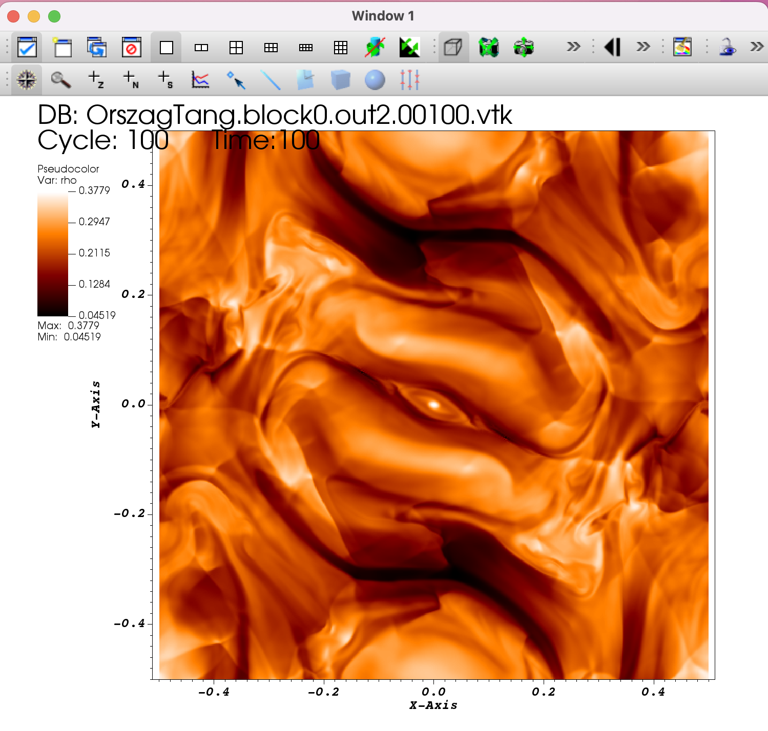
The default grid resolution was 500. As noted above, the grid resolution was set to 200. The following is an image visualized with a grid resolution of 200.
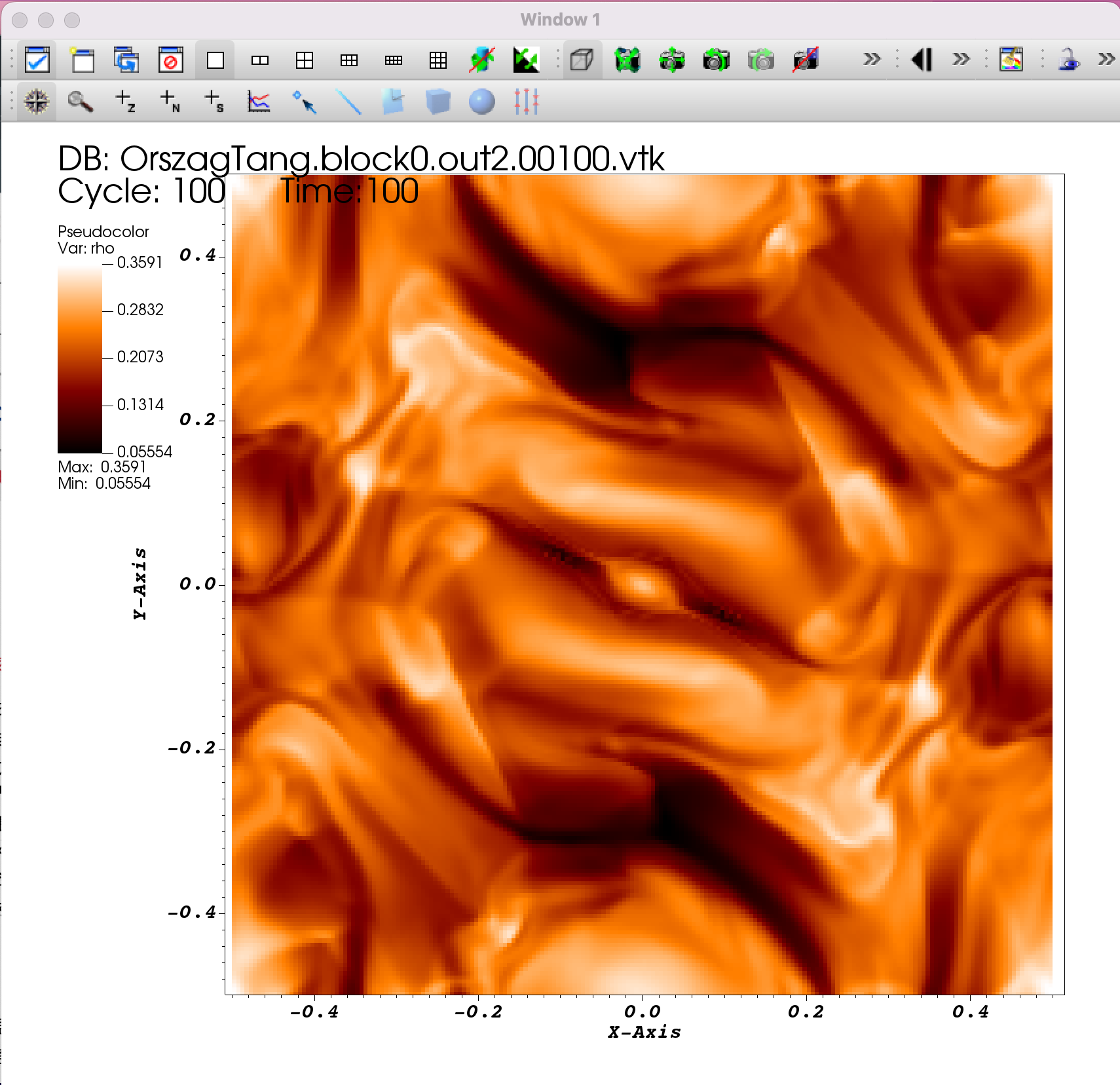
You can see that the resolution is rough compared to the first 500.
Furthermore, the following table compares the execution time (cpu time used) with 250, half of 500.
| number of grids | cpu time use (sec) | cycle | ratio of measured value vs. 500 | theoretical value vs. 500 |
|---|---|---|---|---|
| 500 | 583 | 3563 | - | - |
| 250 | 70 | 1728 | 8.3 | 8.4←2x2x2.1 |
| 200 | 36 | 1368 | 16.2 | 16.3←2.5x2.5x2.6 |
In the above table, “cpu time use” and “cycle” are the output results. The colomn “ratio of measured values vs. 500” is the ratio of 250 and 200 to 500 when the ratio is 1. The theoretical value is the value obtained by multiplying the grid ratio by the ratio of the number of time increments shown in “cycle”.
The measured and theoretical values appear to be in good agreement.