Introduction.
Visualization of 3D magnetohydrodynamic simulation results computed in parallel in this post. The visualization is done with VisIt 3.3.3 running on a Mac.
Visualizing simulation results with VisIt
Environment
The /workdir directory of the docker container with the simulation is under /ext/nfs/athena++ on the physical workstation where the container is running. See the -v option in “Starting Docker” in this post.
If you NFS mount the /ext/nfs area of the above workstation from a Mac, you can view the resulting files from VisIt running on a Mac.
Opening the simulation results file
Run visIt on a Mac and open the simulation results file on the NFS mount with “Open”.
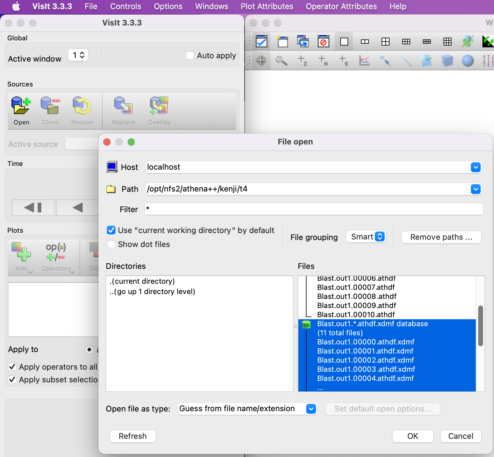
For files, specify Blast.out1.*.athdf.xdmf database and click “OK”.
Open the Expressions file
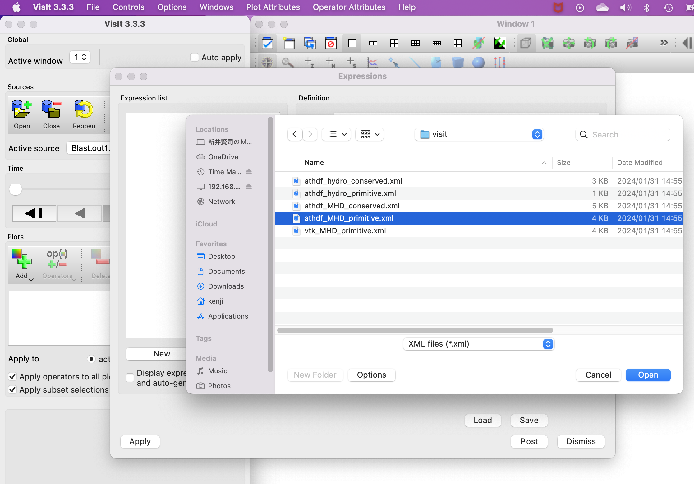
Open the “Controls” → “Expressions” window and click “Load”. Then click “Open” on “athena/vis/visit/athdf_MHD_primitive.xml”.
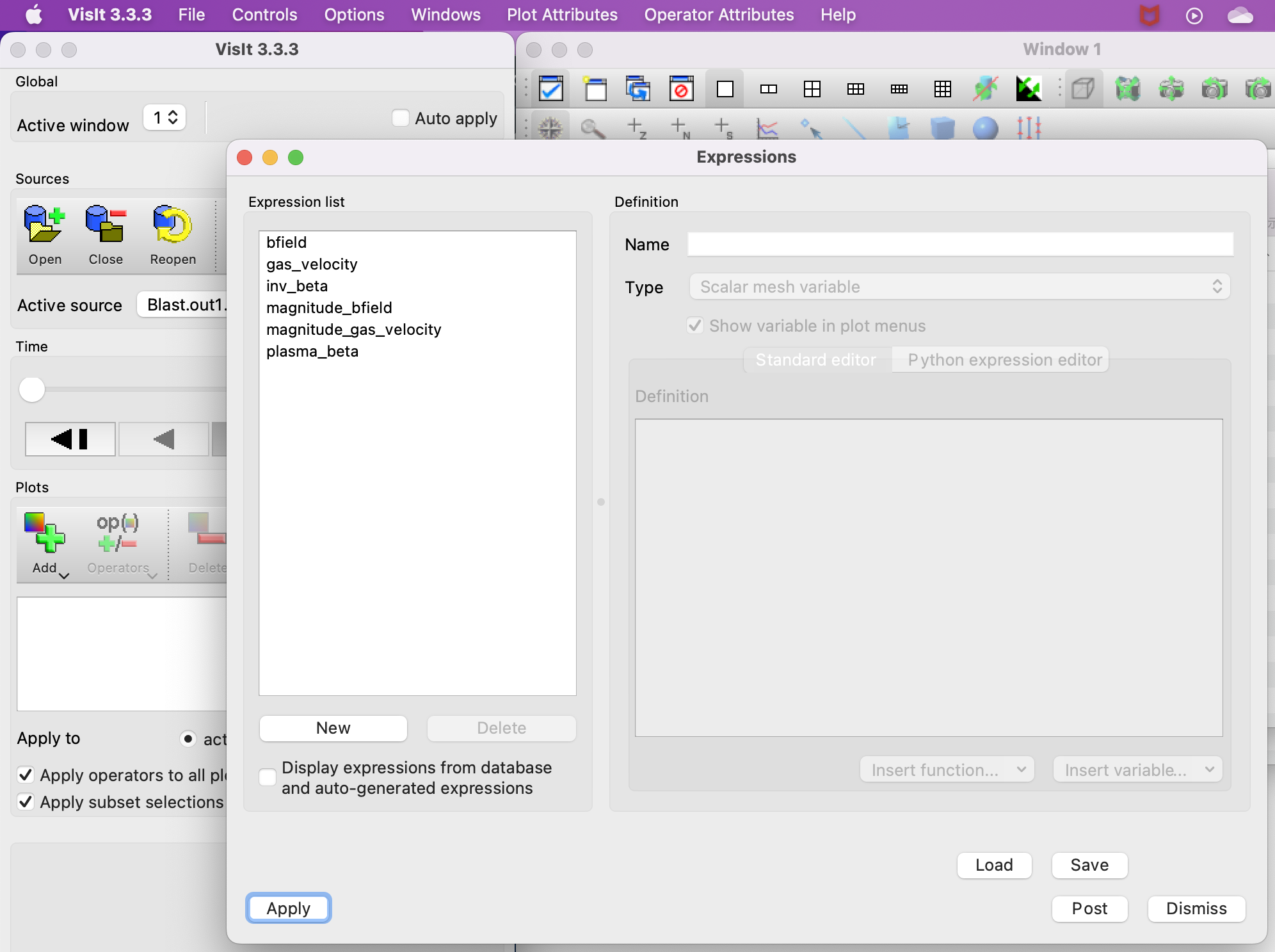
In the “Expressions” window shown below, “Apply” and then click “Dismiss” to close the “Expressions” window.
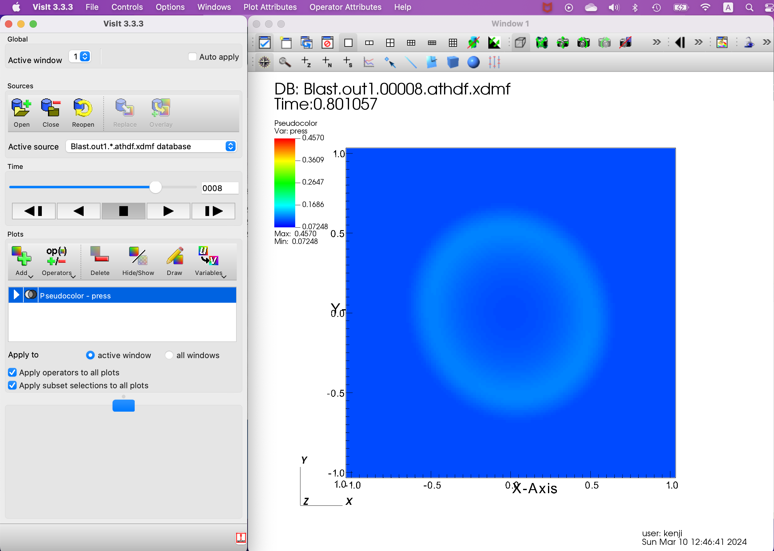
Click “Add” -> “Pseudocolor” -> “press” (no “gas_pressure”), then “Draw”.
The following figure is a screenshot taken a little further in time. In the next section, we will see this cross-section.
Slice Operators
View a cross-section using the “ThreeSlice” operator.
Operator Attributes" → “Slicing” → “ThreeSlice” opens the “ThreeSlice operator attributes” screen (it seems you can specify where to place the cross section, but I’m not sure, so leave the default origin). (I am not sure about this, so I left the default origin as it is.) Click “Apply” to close the “ThreeSlice operator attributes” screen with “Yes, Do not prompt again” and then with “Dismiss” to close the “ThreeSlice operator attributes” screen.
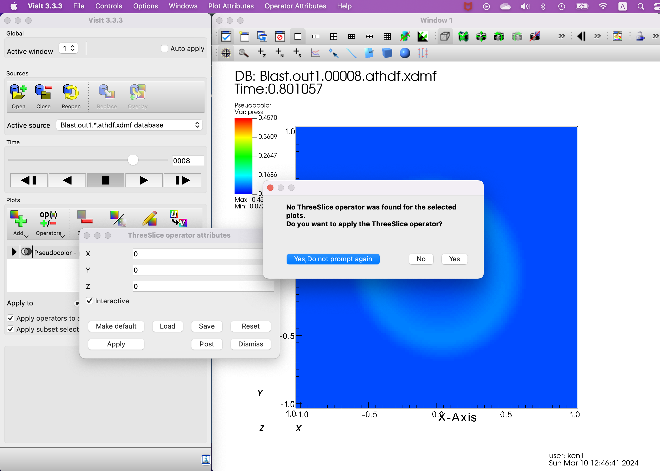
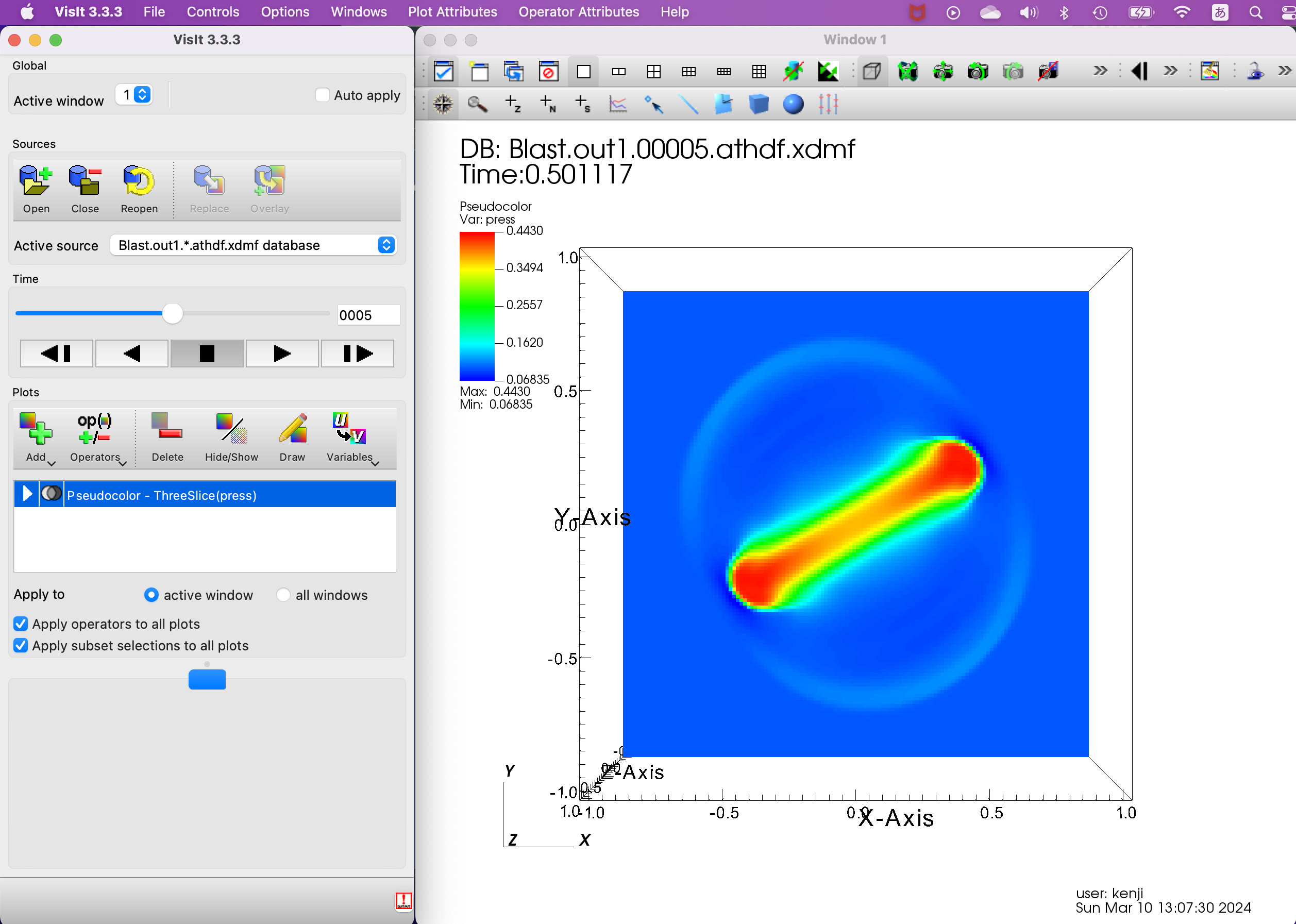
The resulting image is as follows.
velocity vector display
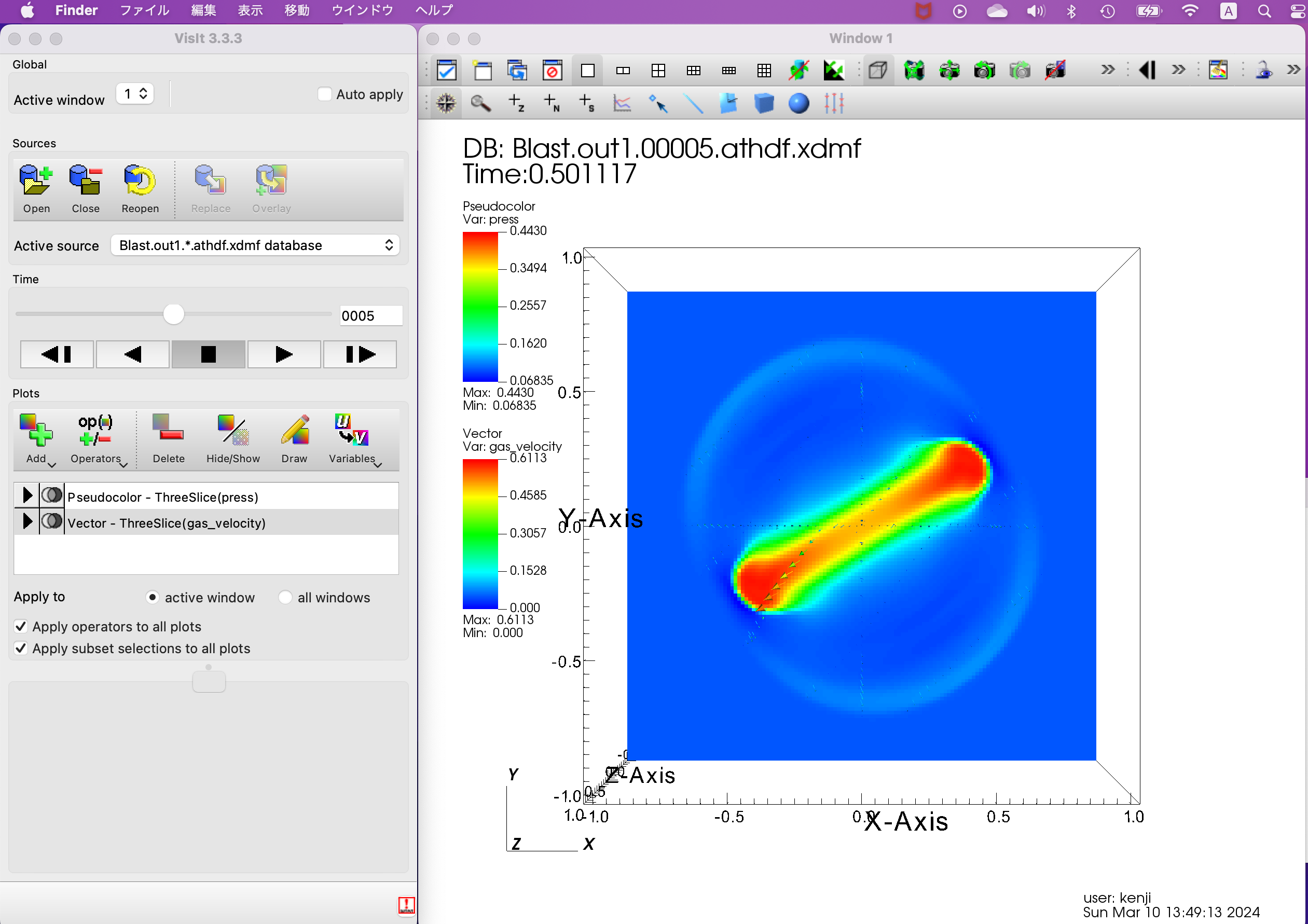
In “Add” → “Vectors” → “gas_velocity”, double-click “gas_volocity” to open the “Vector plot attributes” screen.
Under “Sampling,” change the number of arrows from 400 to 4000 to increase the number of arrows. Under “Geometry,” change the radio button for “Vector origin” to “Middle.
The following figure is thus obtained. Compared with Source 2, there seem to be fewer arrows displayed. The reason is unknown.
Drawing magnetic lines
The next step is to display the magnetic field lines as follows.
Specify “Add” → “Pseudocolor” → “operators” → “IntegralCurve” → “bfield”.
Double-click on IntegralCurve to open the “IntegralCurve operator attributes” (see below).
In the “Integration” tab, change “Source type” to “Plane” and “Normal” to “1 0 0”.
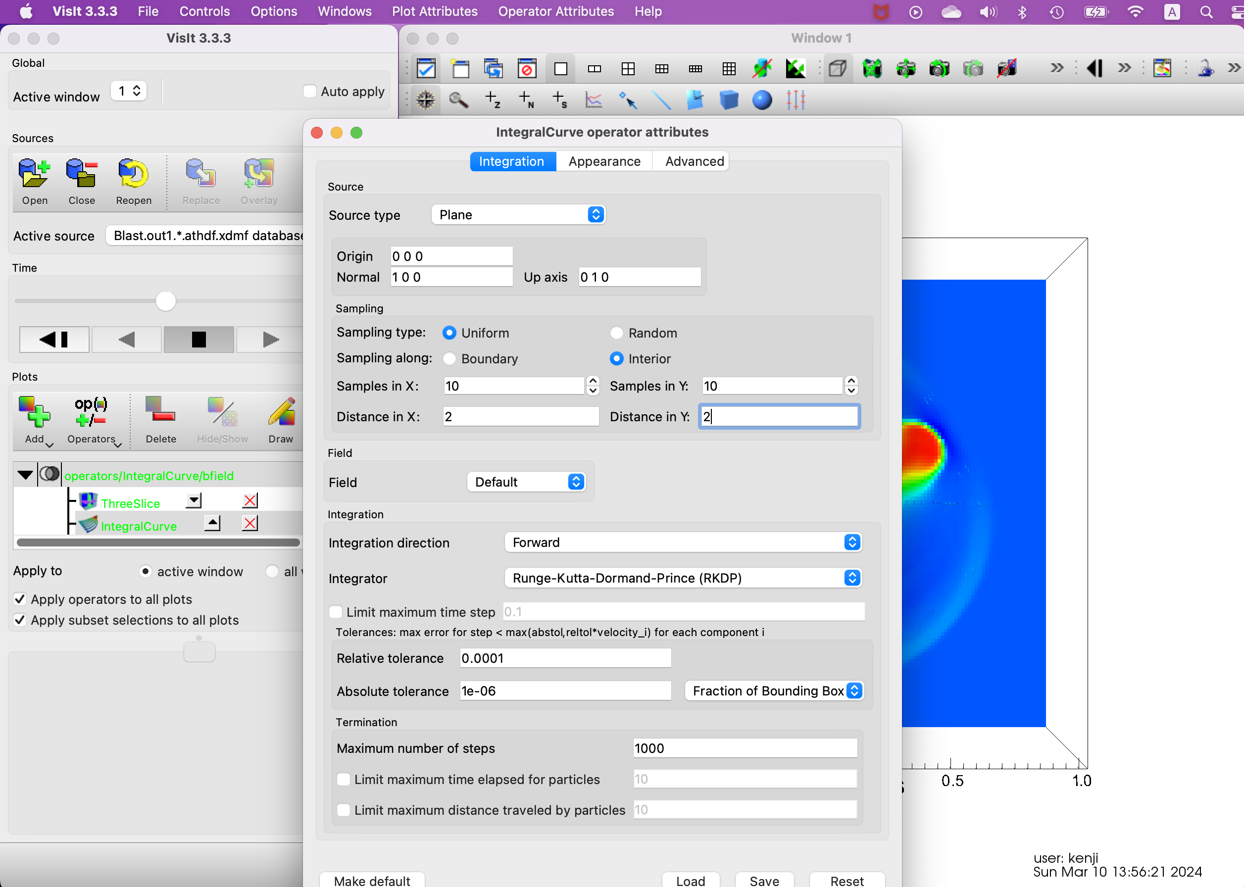
Furthermore, change “Samples in X” and “Samples in Y” to “10” and “Distance in X” and “Distance in Y” to “2”.
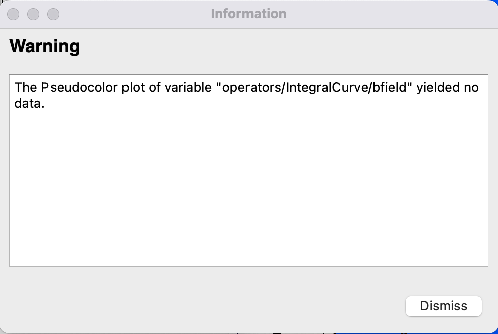
Next, in the “Appearance” tab, specify “Vector magnitude” for “Color by”, “Apply”, “Dismiss”, and “Draw”, the following warning appears and the magnetic field lines are not displayed as in Source 2.
Summary
The visualization of simulation results (calculation results) using VisIt worked well for the most part, but there were some problems with the display of arrows (velocity vectors) and magnetic field lines. In particular, the magnetic field lines were not displayed at all.
I would like to use VisIt to visualize other problems and learn to use VisIt a little more.