Rayleigh-Taylor Instability - Athena++ Tutorial 4 Additional Assignment

Introduction

In this article, I posted about my work on tutorial 4 of Athena++. Here, I post my work on the Rayleigh-Taylor instability challenge in 3D.

Sources.

• Athena Tutorial 4 The Rayleigh-Taylor instability challenge is additional assignment 2 in this tutorial 4. This additional assignment is not on the original page.

Simulation Calculations

Configuration

As before, the docker container was started and configured as follows.

# python configure.py --prob rt -b --flux hlld -mpi -hdf5

As explained in this post, the library designation in the Makefile was changed from “-lhdf5” to “-lhdf5_openmpi”. That was a bit cumbersome, so I tried the following to see if it could be changed with a parameter. For more information, please refer to the original document.

• I added hdf5_openmpi in –lib option. However, I could not disable hdf5 and got a link error.
• I specified the library path with /usr/lib/x86_64-linux-gnu/openmp in -hdf5_path option, but this also failed to disable hdf5 and got a link error.

So I changed configure.py as follows to generate -hdf5_openmpi.

923c923
<         makefile_options['LIBRARY_FLAGS'] += ' -lhdf5_openmpi'
---
>         makefile_options['LIBRARY_FLAGS'] += ' -lhdf5'

make

Here again, as before, I ran make as follows.

# make clean
# make

input file modification

The athena executable created by make and input file (inputs/hydro/athinput.rt3d) were copied to the work area, and athinput.rt3d was edited as follows.

14c14
< file_type  = hdf5       # Binary data dump
---
> file_type  = vtk       # Binary data dump
45,49d44
< <meshblock>
< nx1        = 32         # Number of zones per MeshBlock in X1-direction
< nx2        = 32         # Number of zones per MeshBlock in X2-direction
< nx3        = 32         # Number of zones per MeshBlock in X3-direction
< 
59,60d53
< b0    = 0.0
< angle = 30

First, let’s simulate without magnetic field by setting b0=0.0. Since there is no magnetic field, I assumed that the angle would be ignored, so I left it as it is.

Run

The following command will run the simulation.

# mpirun -np 4 --hostfile myhosts \
-mca plm_rsh_args "-p 12345" \
-mca btl_tcp_if_exclude lo,docker0 \
-oversubscribe $(pwd)/athena \
-i athinput.rt3d > log

Visualization

For a detailed description of visualization, please refer to the previous this article. Here is a brief procedure and a screenshot of the process.

Load the file and display the densities

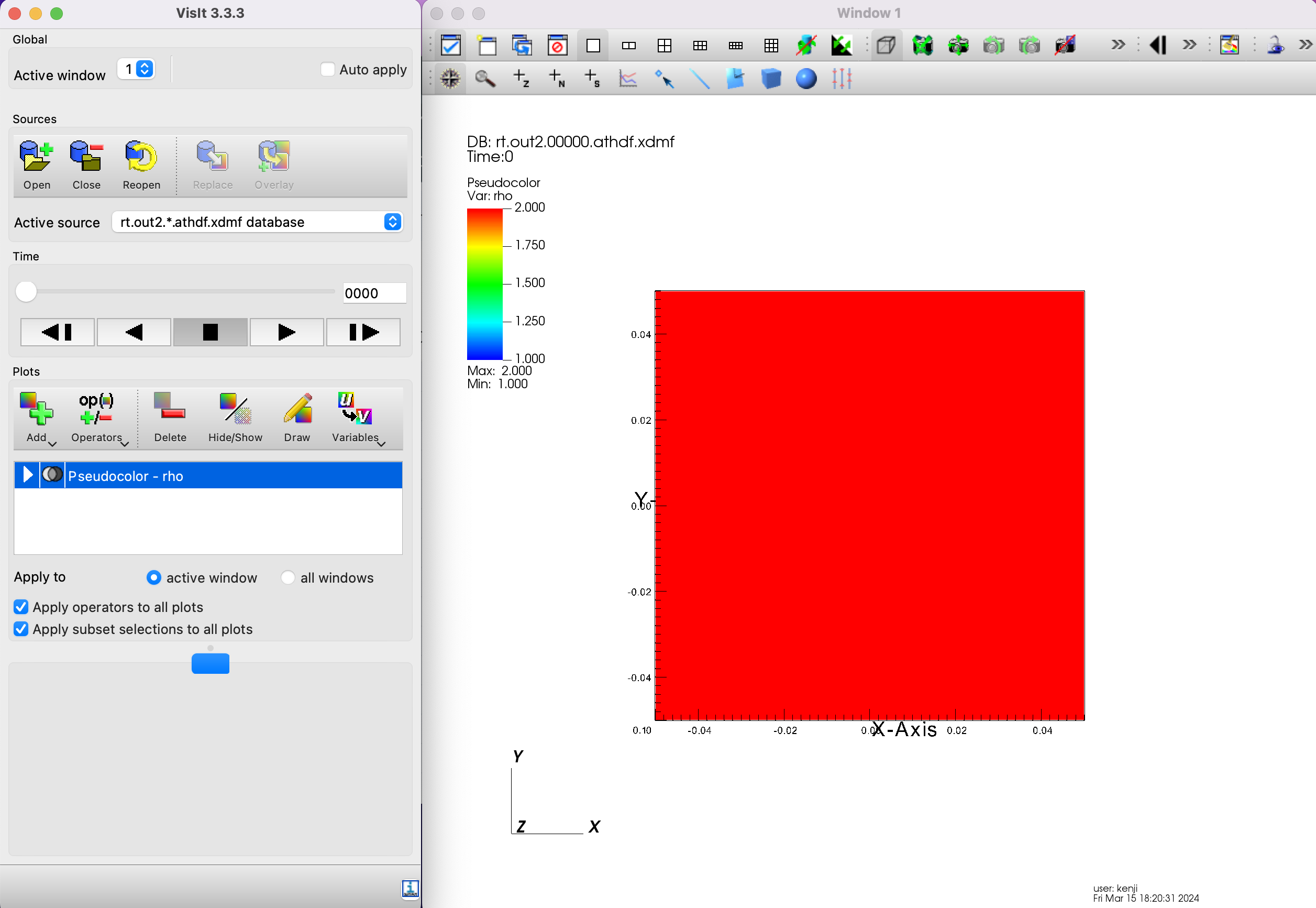
From “Open”, specify the simulation result file rt.out2.*athdf.xdmf database.

Specify “Add” → “Pseudoclor” → “rho” and click (execute) “Draw”.

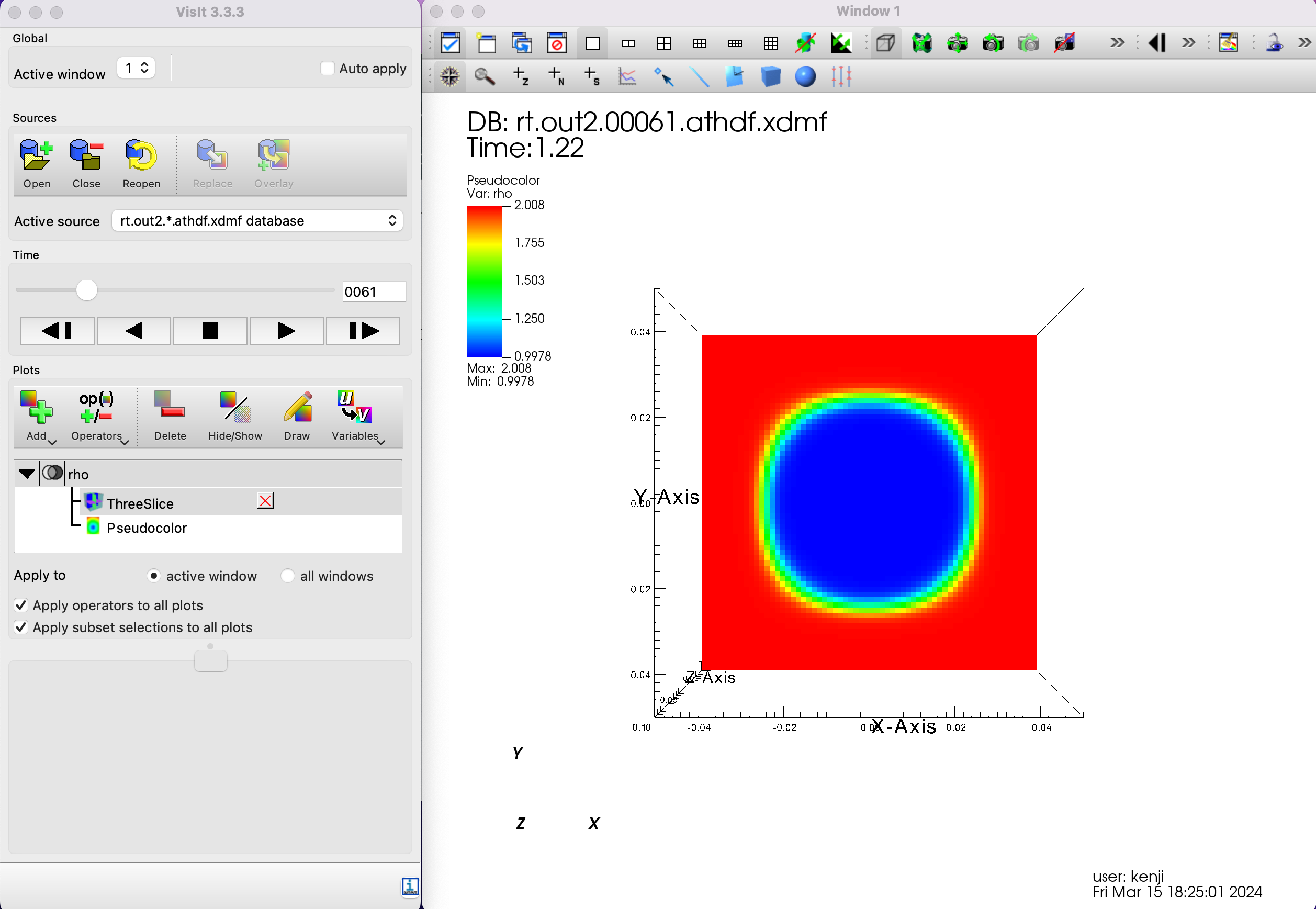
Displaying a cross-section

Specify “Operator Attributes” → “slicing” → “ThreeSlice” and execute “Draw”.

Then, advance the time.

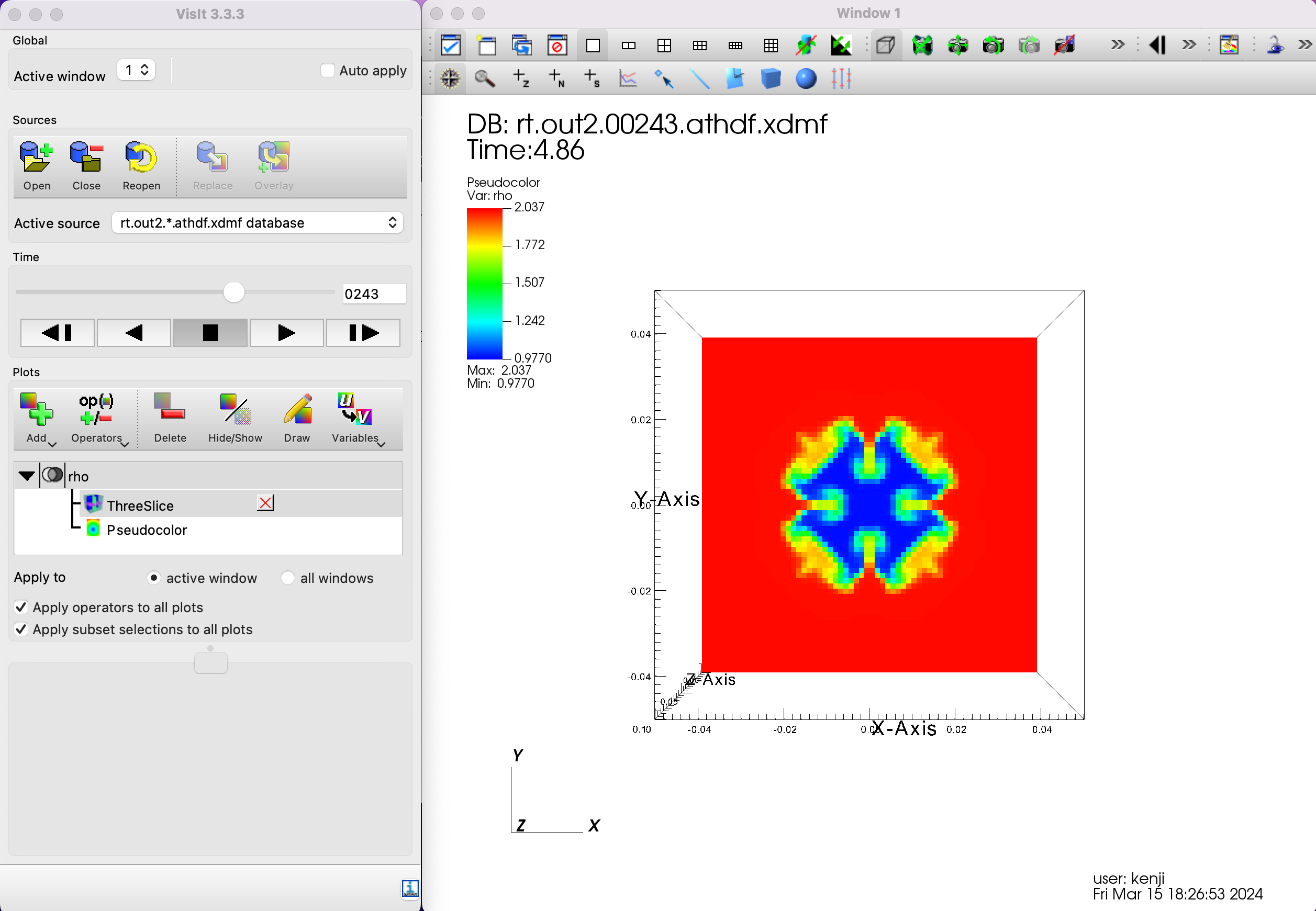
Advance time a bit more; it looks like a cross-section of the typical pattern of Rayleigh-Taylor instability. Let’s display the cross section.

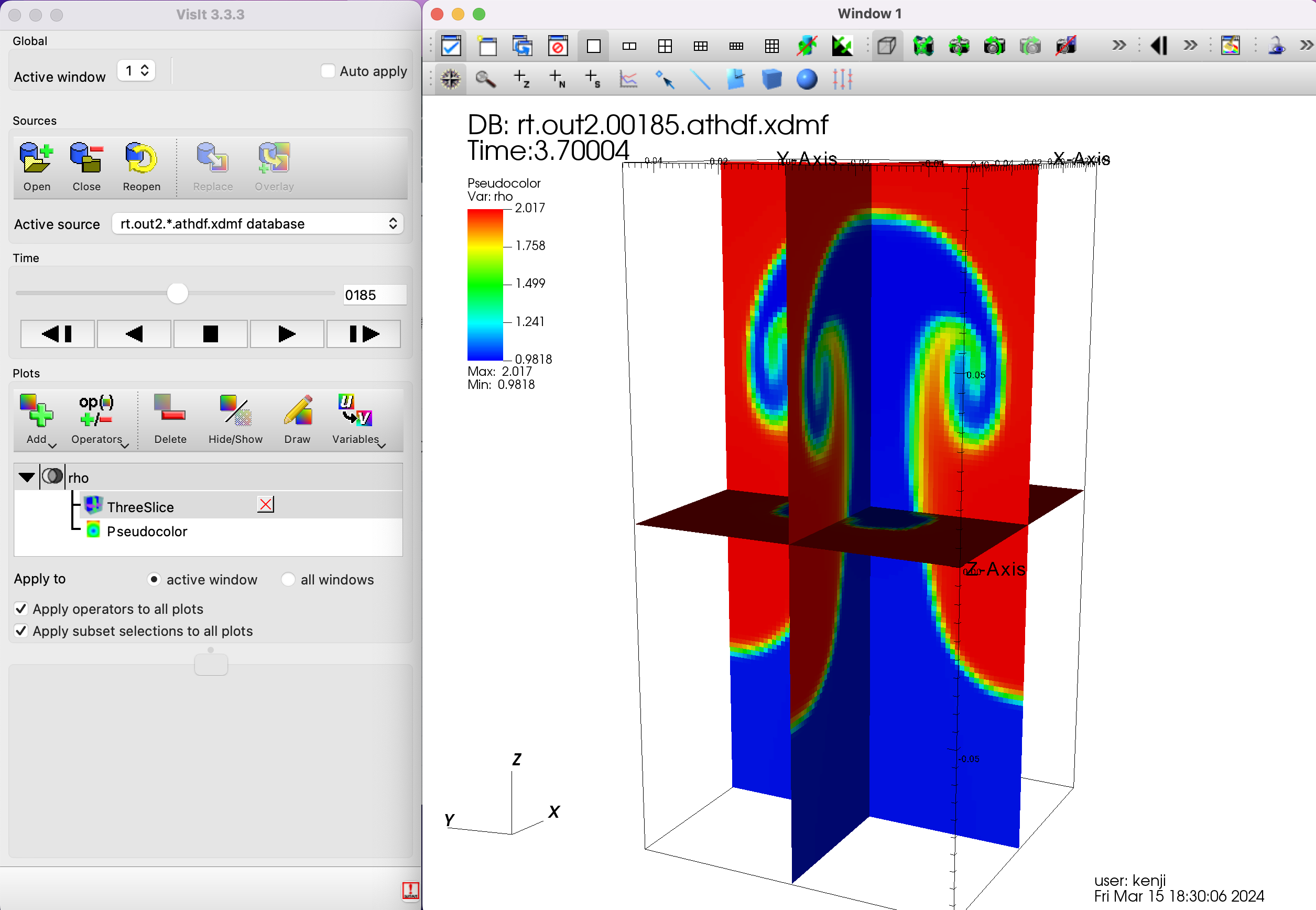
Change the viewpoint.

By holding down the left mouse button and moving it (dragging), you can change the viewpoint. The figure below was obtained by moving back to the time that shows how Rayleigh-Taylor instability.

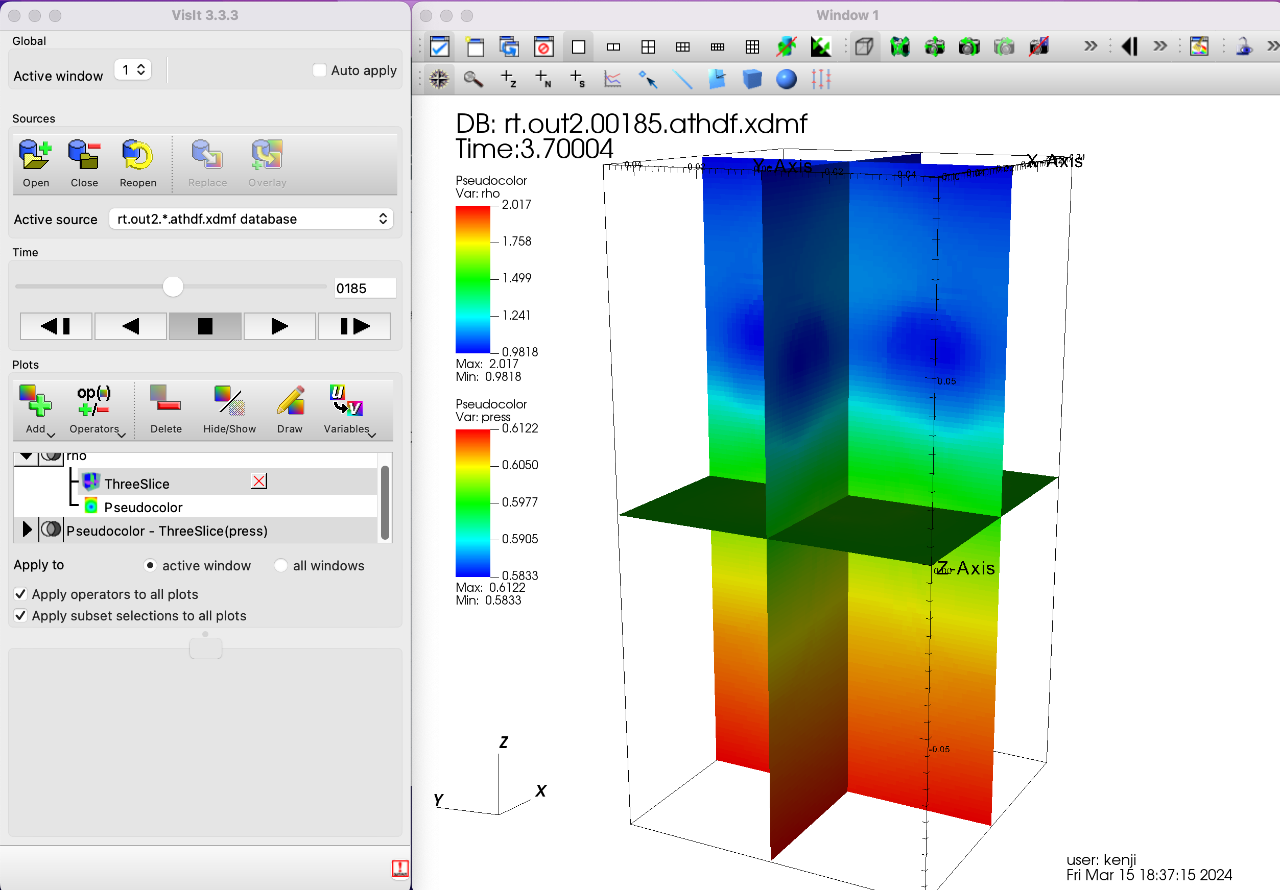
Show the pressure

Now specify “Add” → “Pseudoclor” → “press” and click (execute) “Draw”.

The rho display was once hidden by “Hide/Show”.

For the future

While operating visIt, I am beginning to grasp the quirks (features) of this software. I will try to touch it more freely.

As for Rayleigh-Taylor instability, I will change the initial value or add a magnetic field and see how it goes.