Motivation
I tried PINNs (Physics-Informed Neural Networks) with NVIDIA Modulus over a year ago, After that, it was completely untouched. I have heard Riken/Matsuoka-san’s talk at a recent seminar (AI for Science; here and here), I decided to study it again and tried to implement PINNs using a physically understandable problem as an example.
Sources
- I tried PINNs (Physics Informed Neural Networks) - The page I referred to for implementation aspects. I did not transcribe the code, but coded it by myself after understanding the contents of the code.
- KIT Physical Navigation - I referred to it to understand the differential equations of the mass, spring, and damper model (damped vibration). I understood the path to solving the differential equations by working with my hands, recalling also the solution of the quadratic equation, Euler’s formula, and the additive theorem for trigonometric functions.
- Implementing PINNs (Physics Informed Neural Networks) in Pytorch - A page implementing the same problem (mass, spring, and damper model).
Physical Background
To improve the outlook of the code, the background ideas are summarized below.
Differential Equations
The differential equations representing the mass-spring-damper model are as follows $$ m\frac{d^2x}{dt^2}+c\frac{dx}{dt}+kx=0 \tag{1} $$ Let $m$ be the mass, $c$ be the damping coefficent, and $k$ be the spring constant.
Letting $\gamma=\frac{c}{2m}$ and $\omega_0=\sqrt{\frac{k}{m}}$, equation (1) is as follows. $$ \frac{d^2x}{dt^2} + 2\gamma\frac{dx}{dt}+\omega_0^2x=0 \tag{2} $$ Solving equation (2) (see source 2.) yields $$ x= \exp^{-\gamma t}(A_1\cos \omega t+A_2 \sin\omega t) \tag{3} $$ where $\omega=\sqrt{\omega_0^2 - \gamma^2}$, as boundary conditions, let $x_0$ be the position at $t=0$ and $v_0$ be the velocity, then $A_1= x_0$ and $A_2=\frac{x_0\gamma+v_0}{\omega}$.
for Finite Difference Method(FDM)
From equation (1), if $a_i$ is the acceleration at a certain point in time, it can be expressed as $$ a_i=-\frac{c v_i+k x_i}{m} \tag{4} $$ Velocities and displacements are as follows $$ x_{i+1} = x_i + \frac{dx}{dt}\Delta t \tag{5} $$
$$ v_{i+1} = v_i + \frac{dv}{dt}\Delta t \tag{6} $$
Concept of Loss Function
The loss function, which represents the error with the observed data (in this case, five were chosen from the exact solution), is as follows $$ L_{obs} = \frac{1}{M}\sum_{i}^{m} (M_{pinn}(t_i)-O(t_i))^2 \tag{7} $$ where $M_{pinn}(t_i)$ is the inference result using the model, $O(t_i)$ is the observed data, and $M$ is the number of observed data. Equation (7) is the same as the mean squared error (MSE) when training a normal model.
Next, the loss function for the physical error (error with the differential equation) is as follows. $$ L_{pinn} = \frac{1}{N}\sum_{j}^{n}(f(t_j))^2 \tag{8} $$ where $f(t_j)$ is a differential equation for a physical phenomenon and $N$ is the number of ticks in a certain time segment. Equation (8) works in the direction of establishing the differential equation (1).
The loss function in this case is expressed by the combination of (7) and (8). $$ L_{total} = L_{obs} + \lambda_1 L_{pinn} \tag{9} $$ where $\lambda_{1}$ is a weighting parameter for the error in the observed data and the error from the differential equation.
Code and results
Finite Difference Method
# Finite Diffrence Method
import numpy as np

def FiniteDiff(m, c, k, x0, v0, ts):
    """
    Input:
    m: mass [Kg]
    c: damping coefficent [N.s/m]
    k: spring constant [N/m]
    x0: initial position [m]
    v0: initial velocity [m/s]
    ts: list of time step [s]

    Output:
    x: list of potision at each time step [m]
    """
    x = np.zeros_like(ts)
    v = np.zeros_like(ts)

    x[0] = x0
    v[0] = v0
    dt = ts[1] - ts[0]

    for i in range(len(ts)-1):
        a = -(c*v[i] + k*x[i])/m
        v[i+1] = v[i] + a*dt
        x[i+1] = x[i] + v[i+1]*dt

    return x
Analytical solution
# Analytical Solution

def AnalyticalSol(m, c, k, x0, v0, ts):
    g = c/(2*m)  # gamma
    w0 = np.sqrt(k/m)  # omega 0
    w = np.sqrt(w0*w0 - g*g)
    A1 = x0
    A2 = (x0*g + v0)/w
    x = np.exp(-g*ts) * (A1*np.cos(w*ts) + A2*np.sin(w*ts))

    return x
Initial value
# Initial values

m = 1.0
c = 0.4
k = 10.0
x0 = 1.0
v0 = 0.0
elasped_t = 10.0
n_step = 1000

ts = np.linspace(0, elasped_t, n_step)
Obtain FDM and analytical solutions then Draw graphs
# Solve the problem using Finite Difference Method and analytical solution

x_fd = FiniteDiff(m, c, k, x0, v0, ts)
x_as = AnalyticalSol(m, c, k, x0, v0, ts)
# Draw graphs of time-specific deviations from FDM and Analytical Solution

import matplotlib.pyplot as plt

fig = plt.figure(figsize=(12,8))

ax1 = fig.add_subplot(2, 1, 1)
ax1.plot(ts, x_fd, c='b', label='FiniteDiff')
ax1.set_xlabel('time step', fontsize='14')
ax1.set_ylabel('deviations', fontsize='14')
ax1.set_title('FDM: time-specific deviations', fontsize='18')
ax1.grid()
ax1.legend(fontsize='14')

ax2 = fig.add_subplot(2, 1, 2)
ax2.plot(ts, x_as, c='g', label='AnalyticalSol')
ax2.set_xlabel('time step', fontsize='14')
ax2.set_ylabel('deviations', fontsize='14')
ax2.set_title('Analytical: time-specific deviations', fontsize='18')
ax2.grid()
ax2.legend(fontsize='14')

plt.tight_layout()
plt.show()
Graph

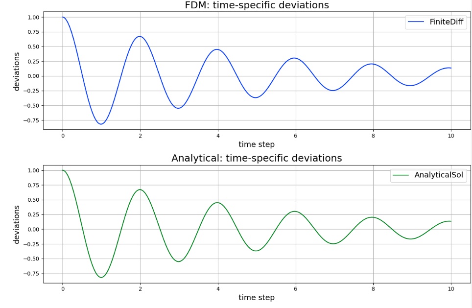
The solution obtained by FDM is consistent with the analytical solution.
Function to graphically display intermediate results
# Evaluate the model at the appropriate epoch

import matplotlib.pyplot as plt

# Inference using the model trained up to this time
# And draw the results of inference at all times in a graph
def EvalModel(model, t_step, t_data, x_data, epoch):
    # Inference
    x_pred = model(t_step)
    x_pred = x_pred.view(1, -1)[0].to("cpu").detach().numpy()

    # Draw a graph
    fig = plt.figure(figsize=(12,4))
    ax1 = fig.add_subplot(1, 1, 1)
    ax1.plot(ts, x_pred, c='r', label='PINNs')
    ax1.scatter(t_data.to("cpu"), x_data.to("cpu"), label='Training data')
    ax1.set_xlabel('time step', fontsize='14')
    ax1.set_ylabel('deviations', fontsize='14')
    ax1.set_title('PINNs: time-specific deviations at '+str(epoch+1)+' epoch', fontsize='18')
    ax1.grid()
    ax1.legend(fontsize='14')
    plt.tight_layout()
    plt.show()
Define model
# Define fully-connected layer Neural network
#  Input layer: 1
#  Hidden layer: 16, 32, 16
#  Output layer: 1

import torch
from torch import nn
import torch.nn.functional as F

class Net(nn.Module):
    def __init__(self):
        super().__init__()
        self.fc1 = nn.Linear(1, 16)  # fully-connected layer
        self.fc2 = nn.Linear(16, 32)
        self.fc3 = nn.Linear(32, 16)
        self.fc4 = nn.Linear(16, 1)

    def forward(self, t):
        x = F.tanh(self.fc1(t))
        x = F.tanh(self.fc2(x))
        x = F.tanh(self.fc3(x))
        x = self.fc4(x)
        return x


# run on cuda if possible
device = 'cuda' if torch.cuda.is_available() else 'cpu'
model = Net().to(device)
Define loss function and optimization function
from torch import optim

# Loss function: Mean Square Error
loss_func = nn.MSELoss()

# Adam
optimizer = optim.Adam(model.parameters(), lr=1e-3)
Prepare observation data and time data for all time domain for PINNs
As observation data, five t_data, indicated by “select_data,” were selected from all time segments (1000 data), and x_data were selected from the exact solution, x_as. The t_pinn was prepared as the data for all time segments for determining the error of the differential equation.
# Prepare data

# Select 5 points from 0 to n_steps-1
#select_data = [0, 200, 500, 700, 900]
#select_data = [0, 150, 250, 350, 550]
select_data = [0, 100, 200, 300, 400]


t_data = torch.tensor(ts[select_data], dtype=torch.float32).view(-1, 1).to(device)
x_data = torch.tensor(x_as[select_data], dtype=torch.float32).view(-1, 1).to(device)

# Prepare time-step data all-over for PINNs

#t_pinn = torch.linspace(0, elasped_t, pinn_step, requires_grad=True).view(-1, 1).to(torch.float32).to(device)
t_pinn = torch.tensor(ts, dtype=torch.float32, requires_grad=True).view(-1, 1).to(device)
Learning Loop
For the parameters discussed in “The Concept of Loss Functions,” we first ran it with $1$.
# Train by Physic informed neural network

lambda1 = 1  # weight of physical error (vs. observed data)
epochs = 50000

record_loss = []

for i in range(epochs):
    # 勾配を0に
    optimizer.zero_grad()

    # 順伝播
    x_pred = model(t_data)
    loss1 = loss_func(x_pred, x_data)

    # Calculate physical formulas(differential equation)
    x_pinn = model(t_pinn)

    x_t = torch.autograd.grad(
        x_pinn,
        t_pinn,
        grad_outputs=torch.ones_like(x_pinn),
        retain_graph=True,
        create_graph=True,
    )[0]
    x_tt = torch.autograd.grad(
        x_t,
        t_pinn,
        grad_outputs=torch.ones_like(x_pinn),
        retain_graph=True,
        create_graph=True,
    )[0]
    f = x_tt + (c/m)*x_t + (k/m)*x_pinn
    loss2 = loss_func(f, torch.zeros_like(f))

    # Calculate the error
    loss = loss1 + lambda1 * loss2
    record_loss.append(loss.item())

    # 逆伝播(勾配を求める)
    loss.backward()

    # Update Parameters
    optimizer.step()

    if i%1000 == 0:
        print("Epoch:", i, "Loss1:", loss1.item(), "loss2:", loss2.item())

    if i%10000 == 0:
        EvalModel(model, t_pinn, t_data, x_data, i)
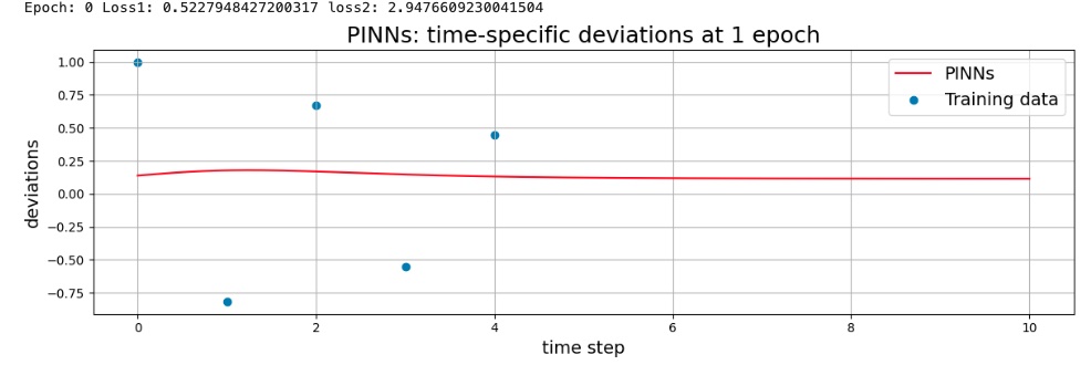
Model after 1 epoch (graph of inference results)

Model after 50,000 epoch (graph of inference results)

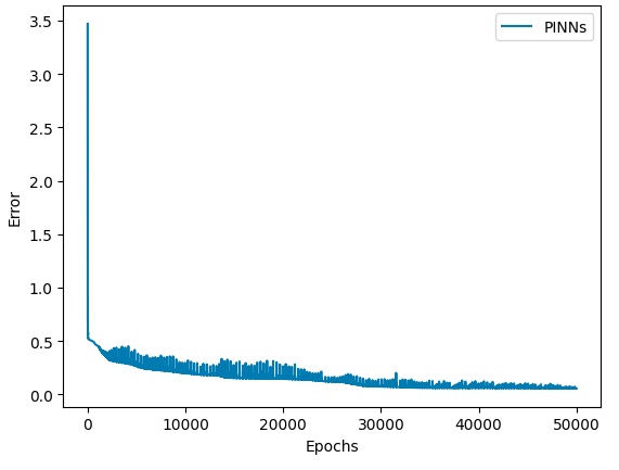
Error convergence status

Review the parameter
Change the parameter
As the training proceeded, it changed to fit the observed values (exact data), but did not perfectly match the observed values even after 5,000 turns. In addition, after 5 seconds without observed values, the decay was rapid, and it was not the same as the decay of the exact solution.
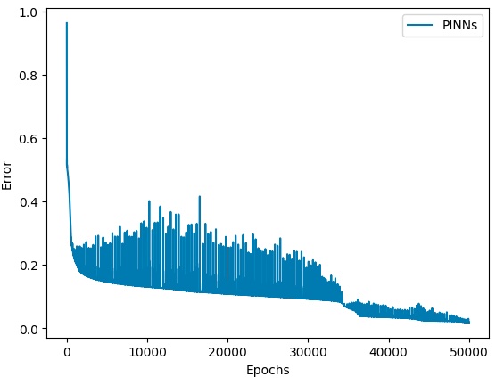
Therefore, in order to weaken the effect of physical errors, the parameter $\lambda_{1}$ was set to $0.2$ to bring it closer to the observed values.
Model after 50,000 epoch (graph of inference results)

Error convergence status

Conclusion
Although I’ve understood a little better the concept of PINNs, the results of inference using a model trained 50,000 times with PINNs did not match the analytical solution. The code was reviewed many times, but the cause is unknown at this time.
Maybe I will know if I try another problem with PINNs to understand it further.