PINNs

Introduction

Recently, I summarized the mass, spring, and damper problem with PINNs. This time, I’ve worked on the Burgers’ equation and summarized it.

Sources.

.Solving 1D Burgers’ Equation - Finite Difference vs Neural Network - FDM ( This page solves the Burgers’ equation using two methods: Finite Difference Method and PINNs. This page was very helpful this time.
Implementing Physics-Informed Neural Networks with Pytorch (1) Burgers Equation - I referred to the code for the PINNs implementation aspect. Plotting the initial state is largely due to this page.
pinn_burgers - This page uses the memory-restricted BFGS method (the BFGS method is one of the quasi-Newtonian solution methods) as an optimizer.
Physics Informed Deep Learning (Part I) - A paper on the effectiveness of PINNs. Also referenced from source 3. Here is Part II. I have not read Part I or Part II myself.

Physical Background

To understand the code, I first summarize the physical background. Although it lacks mathematical rigor, I believe I have organized the main points.

Differential Equations

Considering the field represented by $u(x, t)$ and letting $\nu$ be the kinematic viscosity, the Burgers’s equation is given by $$ \frac{\partial u}{\partial t} + u\frac{\partial u}{\partial x} =\nu\frac{\partial^{2}u}{\partial x^{2}} \tag{1} $$

Finite Difference Method

First, in the function $f(x)$, Taylor series with $x+\Delta x$ and $x-\Delta x$ can be expressed as follows. $$ f(x+\Delta x)=f(x)+\frac{\partial f(x)}{\partial x}\Delta x +\frac{1}{2!}\frac{\partial^{2}f(x)}{\partial x^{2}}\Delta x^{2} + \frac{1}{3!}\frac{\partial^{3}f(x)}{\partial x^{3}}\Delta x^{3} + \cdots \tag{2} $$ $$ f(x-\Delta x)=f(x)-\frac{\partial f(x)}{\partial x}\Delta x +\frac{1}{2!}\frac{\partial^{2}f(x)}{\partial x^{2}}\Delta x^{2} - \frac{1}{3!}\frac{\partial^{3}f(x)}{\partial x^{3}}\Delta x^{3} + \cdots \tag{3} $$

With reference to equations (2) and (3), for the function $u(x,t)$, $u_{i-1}, u_i, u_{i+1}$ can be written as follows. $$ u_{i+1} = u_i + \Delta x \frac{\partial u}{\partial x} |_i + \frac{\Delta x^2}{2}\frac{\partial^2 u}{\partial x^2}|_i + \frac{\Delta x^3}{6}\frac{\partial^3 u}{\partial x^3}|_i + \mathcal{O}(\Delta x^4) \tag{4} $$ $$ u_{i-1} = u_i - \Delta x \frac{\partial u}{\partial x} |_i + \frac{\Delta x^2}{2}\frac{\partial^2 u}{\partial x^2}|_i - \frac{\Delta x^3}{6}\frac{\partial^3 u}{\partial x^3}|_i + \mathcal{O}(\Delta x^4) \tag{5} $$

The sum of equations (4) and (5) is $$ u_{i-1}+u_{i+1} = 2u_i +\Delta x^2\frac{\partial^2 u}{\partial x^2}|_i + \mathcal{O}(\Delta x^4) \tag{6} $$ Ignoring higher-order terms, we can derive $$ \frac{\partial^2 u}{\partial x^2} = \frac{u_{i-1} - 2u_i + u_{i+1}}{\Delta x^2} \tag{7} $$ where the time derivative of the physical quantity $u$ is defined as the limit of $$ \frac{\partial u}{\partial t} = \lim_{\Delta x \rightarrow 0}\frac{u(x+\Delta t)-u(x)}{\Delta t} \tag{8} $$ In equation (8), if $\Delta t$ is a minute quantity, the approximation is as follows $$ \frac{\partial u}{\partial t} \approx \frac{u(x+\Delta t)-u(x)}{\Delta t} \tag{9} $$ The Burgers’ equation (1) can be expressed discretely using equations (7) and (9) as follows $$ \frac{u_i^{n+1} - u_i^n}{\Delta t} + u_i^n\frac{u_i^n - u_{i-1}^n}{\Delta x} = \nu\frac{u_{i+1}^n -2u_i^n + u_{i-1}^n}{\Delta x^2} \tag{10} $$ where $u^{n+1}$ denotes the function when time advances by one from $u^n$.

Equation (10) is solved in $u_i^{n+1}$ as follows $$ u_i^{n+1} = u_i^n - u_i^n\frac{\Delta t}{\Delta x}(u_i^n - u_{i-1}^n) + \frac{\nu \Delta t}{\Delta x^2}(u_{i+1}^n -2u_i^n + u_{i-1}^n) \tag{11} $$ Equation (11) is the formula for advancing from the function value at $u^n$ to the next time step.

Let $NN(x)$ denote the neural network as a function $NN(x)$, and consider the function $NN(x,t)$ to represent the Burgers’ equation.

According to the Universal Approximation Theorem, a neural network can approximate any continuous function, so the Burgers’ equation can be represented by the following neural network. $$ u(x,t) \approx NN(x,t) \tag{12} $$ Let the differential coefficients of the function $NN(x,t)$ be $\frac{\partial NN}{\partial t}, \frac{\partial^2 NN}{\partial x^2}$ etc., then the Burgers equation in (1) is as follows. $$ f(x,t) = \frac{\partial NN}{\partial t} + NN \frac{\partial NN}{\partial x} - \nu \frac{\partial^2 NN}{\partial x^2} = 0 \tag{13} $$ In PINNs, the above is referred to as the governing equation. We will minimize the error in this governing equation.

Code

Import package (library)

# Import packages

import numpy as np

import torch
import torch.nn as nn
import torch.nn.functional as F
from torch import optim
from torch.optim import lr_scheduler

import matplotlib.pyplot as plt
from matplotlib import cm

# run on cuda if possible
device = 'cuda' if torch.cuda.is_available() else 'cpu'

Define constants

# Define constants

# Define the spatio-temporal extent of the problem domain
#    x∈[0,2]  t∈[0,0.48]
x_min = 0
x_max = 2

t_min = 0
t_max = 0.48

x_total = 1000
t_total = 1000

dx = (x_max - x_min)/x_total
dt = (t_max - t_min)/t_total

# kinematic viscosity
k_vis = 0.01/np.pi

# For subsequent calculations, 
# create a grid of the spatio-temporal region in question.

x = torch.linspace(x_min, x_max, x_total).view(-1,1)
t = torch.linspace(t_min, t_max, t_total).view(-1,1)

X, T = torch.meshgrid(x.squeeze(1),t.squeeze(1), indexing='ij')

Define initial and boundary conditions

# Initial condition: u=sin(πx) when t= 0, x∈[0,2]
X_init = torch.hstack((X[:,0][:,None], T[:,0][:,None]))
U_init = torch.sin(np.pi*X_init[:,0]).unsqueeze(1)

# Boundary condition: u=0 when x=0, x=2, t∈[0,0.48]
X_bottom = torch.hstack((X[0,:][:,None], T[0,:][:,None]))
X_top = torch.hstack((X[-1,:][:,None], T[-1,:][:,None]))
U_bottom = torch.zeros(X_bottom.shape[0],1)
U_top = torch.zeros(X_top.shape[0],1)

X_bc = torch.vstack([X_bottom, X_top])
U_bc = torch.vstack([U_bottom, U_top])

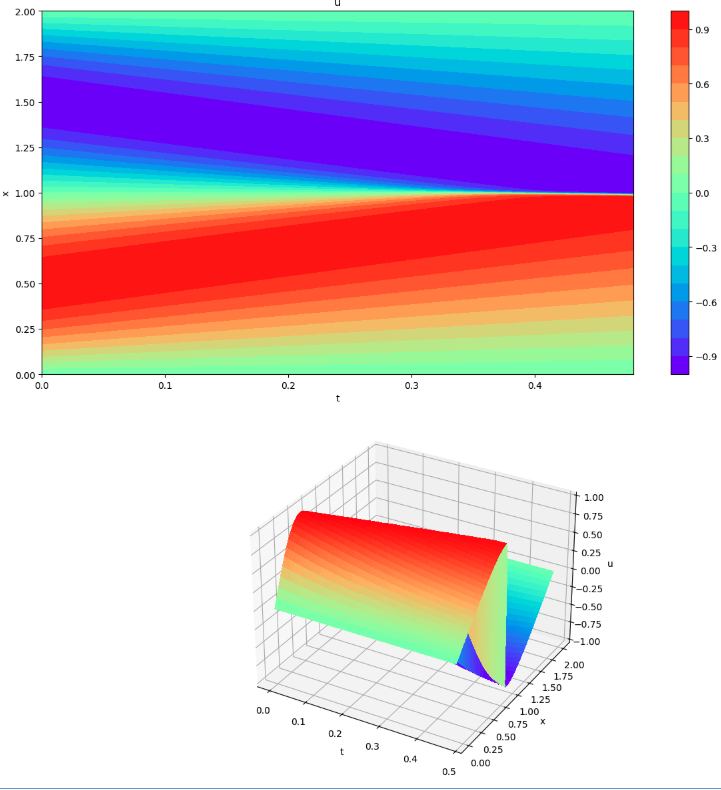
Solving by finite difference method (Visualization 1)

# FDM Function for Burgers' equation

def FDM(st):
    x_num = st.shape[0]
    t_num = st.shape[1]
    for j in range(1, t_num):
        for i in range(1, x_total-1):
            x = st[:,j-1]
            st[i, j] = x[i] - x[i]*(dt/dx)*(x[i]-x[i-1]) + k_vis*dt/(dx*dx)*(x[i+1]-2*x[i]+x[i-1])

# Draw contour plots of u(x,t) for all regions of a given time and space

def plot3d(x, t, u):
    X, T = np.meshgrid(x, t, indexing='ij')
    fig = plt.figure(figsize=(12,12))
    ax1 = fig.add_subplot(2, 1, 1)
    cp = ax1.contourf(T, X, u, 20, cmap=cm.rainbow)
    fig.colorbar(cp)
    ax1.set_title('u')
    ax1.set_xlabel('t')
    ax1.set_ylabel('x')

    ax2 = fig.add_subplot(2, 1, 2, projection='3d')
    surf = ax2.plot_surface(T, X, u, cmap=cm.rainbow, antialiased=False)
    ax2.set_xlabel('t')
    ax2.set_ylabel('x')
    ax2.set_zlabel('u')

    plt.tight_layout()
    plt.show()

# Prepare a 2-dimensional array to store u(x,t)
# And set initial condition
st = np.zeros([x_total, t_total])  # array[space, time]
st[:,0] = U_init[:,0]

# Solve Burgers' equation with Finite Differential Method
FDM(st)

u_fdm = st  # Save for comparison with PINNs

plot3d(X[:,0], T[0,:], st)

Select the part to be used from the initial and boundary conditions.

# Select the number of pieces specified from the initial and boundary conditions

# Define the number of pieces to be selected
N_ic = 1000
N_bc = 1000

idx = np.random.choice(X_init.shape[0], N_ic, replace=False)
X_ic_select = X_init[idx, :].to(device)
U_ic_select = U_init[idx, :].to(device)

idx = np.random.choice(X_bc.shape[0], N_bc, replace=False)
X_bc_select = X_bc[idx, :].to(device)
U_bc_select = U_bc[idx, :].to(device)

初期条件については、「x_total」と「N_ic」の値の関係から分かる通り、当初作成したデータの全てを使用している。

PINNsを評価するためのデータセットを作成

# Create a test set from u(x,t) obtained by FDM
# to evaluate the model in the middle of training
x_test = torch.hstack((X.transpose(1,0).flatten()[:,None],
                       T.transpose(1,0).flatten()[:,None])).to(device)
u_test = torch.from_numpy(u_fdm.transpose(1,0).flatten()[:,None]).float().to(device)

The above data is a test data set to evaluate the model being trained using PINNs. The correct data is the data created by FDM.

Create data for the area to be calculated for PINNs

(13) Create a data set to evaluate(minimize the error) the equation(13) . Eventually, add initial and boundary conditions as well.

# Coordinates of the computational domain
# in which the PINNs' loss is evaluated: x ∈ [0,2], t ∈ [0,0.48]
n_domain = 10000
t_domain = torch.rand(n_domain) * t_max
x_domain = torch.rand(n_domain) * x_max

X_train = torch.stack([x_domain, t_domain], dim=0).T.to(device)

X_train_final = torch.vstack((X_train, X_ic_select, X_bc_select))

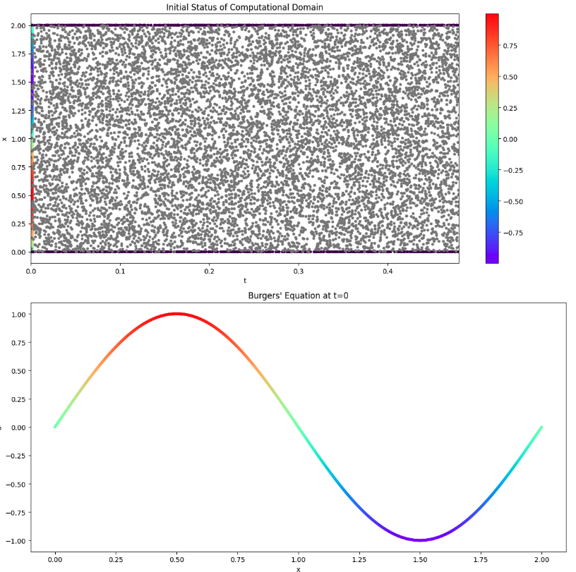
Visualization of initial and boundary conditions and evaluation areas (Visualization 2)

# Graph the status before starting

fig = plt.figure(figsize=(12,12))
ax1 = fig.add_subplot(2, 1, 1)
ax1.set_xlim(t_min, t_max)
ax1.set_title('Initial Status of Computational Domain')
ax1.set_xlabel('t')
ax1.set_ylabel('x')
cp = ax1.scatter(X_ic_select[:,1].to("cpu"), X_ic_select[:,0].to("cpu"), c=U_ic_select.to("cpu"), cmap=cm.rainbow, s=50)  # initial condition
fig.colorbar(cp)
ax1.scatter(X_bc_select[:,1].to("cpu"), X_bc_select[:,0].to("cpu"), c=U_bc_select.to("cpu"), s=10)  # boundary condition
ax1.scatter(X_train[:,1].to("cpu"), X_train[:,0].to("cpu"), c='gray', s=10)  # computational domain

ax2 = fig.add_subplot(2, 1, 2)
ax2.scatter(X_ic_select[:,0].to("cpu"), U_ic_select.to("cpu"), c=U_ic_select.to("cpu"), cmap=cm.rainbow, s=10)
ax2.set_title('Burgers\' Equation at t=0')
ax2.set_xlabel('x')
ax2.set_ylabel('u')

plt.tight_layout()
plt.show()

Define Neural Networks

# define u_NN class

class u_NN(nn.Module):
    def __init__(self, n_input, n_output, n_hiddens=[32,64,128,128,64,32]):
        super().__init__()
        self.activation = nn.Tanh()
        self.input_layer = nn.Linear(n_input, n_hiddens[0])
        self.hidden_layers = nn.ModuleList(
            [nn.Linear(n_hiddens[i], n_hiddens[i+1]) for i in range(len(n_hiddens)-1)]
        )
        self.output_layer = nn.Linear(n_hiddens[-1], n_output)

    def forward(self, x):
        x = self.activation(self.input_layer(x))
        for layer in self.hidden_layers:
            x = self.activation(layer(x))
        x = self.output_layer(x)
        return x

    def loss_bc(self, x_bc, u_bc):
        u_pred = self.forward(x_bc)
        l_bc = loss_func(u_pred, u_bc)
        return l_bc

    def loss_ic(self, x_ic, u_ic):
        u_pred = self.forward(x_ic)
        l_ic = loss_func(u_pred, u_ic)
        return l_ic

    def loss_pinn(self, x):
        x_clone = x.clone()
        x_clone.requires_grad = True

        NN = self.forward(x_clone)
        NNx_NNt = torch.autograd.grad(
            NN,
            x_clone,
            torch.ones([x_clone.shape[0], 1]).float().to(device),
            retain_graph=True,
            create_graph=True,
        )[0]
        NNxx_NNtt = torch.autograd.grad(
            NNx_NNt,
            x_clone,
            torch.ones(x_clone.shape).float().to(device),
            create_graph=True,
        )[0]
        NNt = NNx_NNt[:,[1]]  # dt term
        NNx = NNx_NNt[:,[0]]  # dx term
        NNxx = NNxx_NNtt[:,[0]]  # dx^2 term

        f = NNt + self.forward(x_clone)*(NNx) + k_vis*NNxx

        zeros = torch.zeros(f.shape[0],1).float().to(device)
        l_pinn = loss_func(f, zeros)
        return l_pinn

    def total_loss(self, x_ic, u_ic, x_bc, u_bc, x):
        l_bc = self.loss_bc(x_bc, u_bc)
        l_ic = self.loss_ic(x_ic, u_ic)
        l_pinn = self.loss_pinn(x)
        return l_bc+l_ic+l_pinn


PINN = u_NN(2, 1).to(device)

The part for finding the differential coefficient of “loss_pinn” was not coded well by me, so I used it from source 1.

I think above part is the key part of this issue.

The structure of the defined model is as follows.

u_NN(
  (activation): Tanh()
  (input_layer): Linear(in_features=2, out_features=32, bias=True)
  (hidden_layers): ModuleList(
    (0): Linear(in_features=32, out_features=64, bias=True)
    (1): Linear(in_features=64, out_features=128, bias=True)
    (2): Linear(in_features=128, out_features=128, bias=True)
    (3): Linear(in_features=128, out_features=64, bias=True)
    (4): Linear(in_features=64, out_features=32, bias=True)
  )
  (output_layer): Linear(in_features=32, out_features=1, bias=True)
)

Define error function, optimizer

from torch import optim

# Loss function: Mean Square Error
loss_func = nn.MSELoss()

# Optimizer: Adam(Adaptive moment estimation)
optimizer = optim.Adam(PINN.parameters(), lr=0.001)

scheduler = lr_scheduler.ExponentialLR(optimizer, gamma=0.98)

Learning loop

# Learning Loop

num_epoch = 20000  # epoch count

# List Variables for Recording
Epoch = []
Learning_Rate = []
IC_loss = []
BC_loss = []
PINN_loss = []
Total_loss = []
Test_loss = []

for i in range(num_epoch):
    if i == 0:
        print("Epoch \t Learning-Rate \t IC_Loss \t BC_Loss \t PINN_Loss \t Total_Loss \t Test_Loss")
        
    l_ic = PINN.loss_ic(X_ic_select, U_ic_select)
    l_bc = PINN.loss_bc(X_bc_select, U_bc_select)
    l_pinn = PINN.loss_pinn(X_train_final)
    loss = PINN.total_loss(X_ic_select, U_ic_select, X_bc_select, U_bc_select, X_train_final)

    optimizer.zero_grad()
    loss.backward()
    optimizer.step()

    if i % 100 == 0:
        with torch.no_grad():
            test_loss = PINN.loss_bc(x_test,u_test)
            Epoch.append(i)
            Learning_Rate.append(scheduler.get_last_lr()[0])
            IC_loss.append(l_ic.detach().cpu().numpy())
            BC_loss.append(l_bc.detach().cpu().numpy())
            PINN_loss.append(l_pinn.detach().cpu().numpy())
            Total_loss.append(loss.detach().cpu().numpy())
            Test_loss.append(test_loss.detach().cpu().numpy())

        if i % 1000 == 0:
            print(i, "\t",
                  format(scheduler.get_last_lr()[0], ".4E"), "\t",
                  format(l_ic.detach().cpu().numpy(), ".4E"), "\t",
                  format(l_bc.detach().cpu().numpy(), ".4E"), "\t",
                  format(l_pinn.detach().cpu().numpy(), ".4E"), "\t",
                  format(loss.detach().cpu().numpy(), ".4E"), "\t",
                  format(test_loss.detach().cpu().numpy(), ".4E"), "\t",
                 )
        scheduler.step()

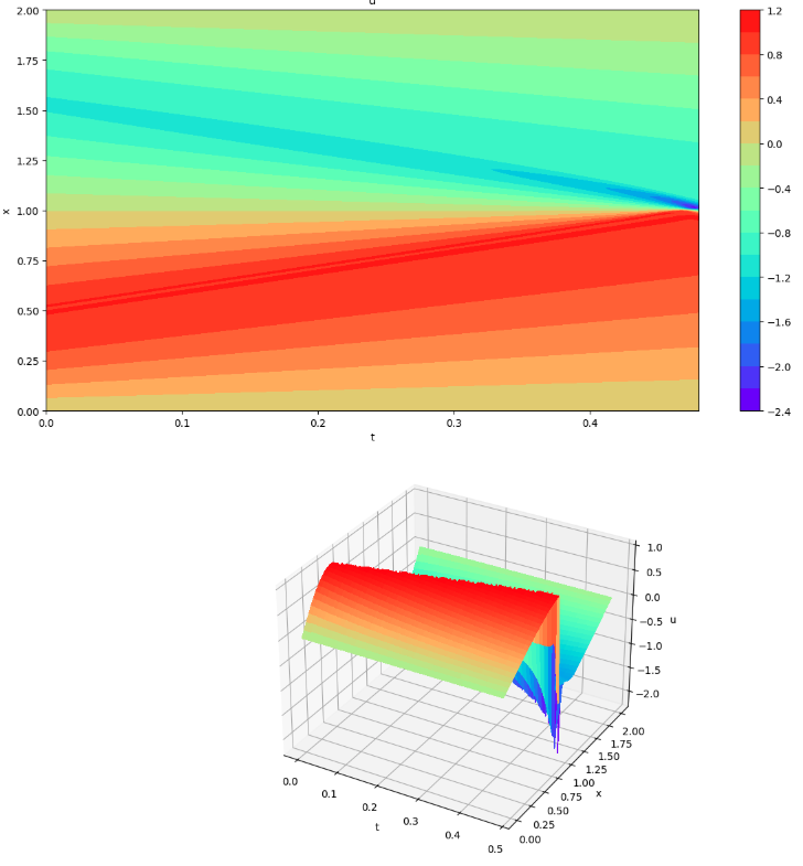
Evaluate the learned model (visualization 3)

# Inference the entire domain of a given time and space
# using the model learned for evaluation

x_mesh = np.linspace(x_min, x_max, x_total)
t_mesh = np.linspace(t_min, t_max, t_total)
X_mesh, T_mesh = np.meshgrid(x_mesh, t_mesh)

# Inference
X = X_mesh.reshape(-1, 1)
T = T_mesh.reshape(-1, 1)
Y = np.block([X, T])
Y = torch.tensor(Y, requires_grad=True, dtype=torch.float32).to(device)
U = PINN(Y)
st = U.view(-1, 1).to("cpu").detach().numpy()
st = np.reshape(st, (t_total, x_total)).T  # Transposition as it can be packed in the column direction.

I got into a bit of a bind when reshaping the “U” (column vector), the result of the inference, into a 2-dimensional “st”, not realizing that it would be filled in the column direction and forgetting to transpose it.

# Draw contour plots of u(x,t) for all regions of a given time and space
# using trained model

u_pinn = U.reshape(t_total,x_total).T.detach().to("cpu").numpy()
plot3d(x_mesh, t_mesh, u_pinn)

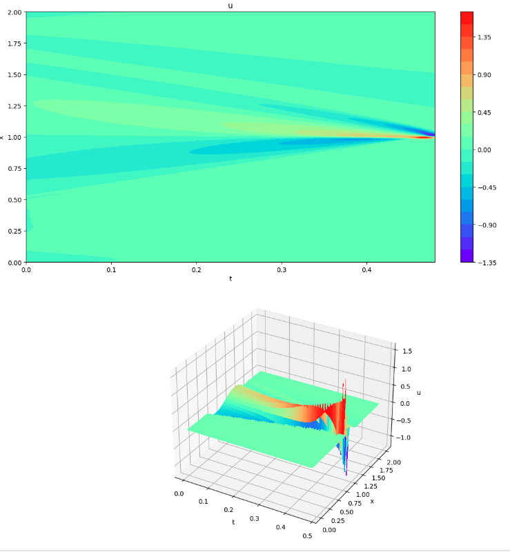
Differences between PINNs and FDMs (Visualization 4)

# Displays the difference between FDM and PINNs
plot3d(x_mesh, t_mesh, (u_pinn-u_fdm))

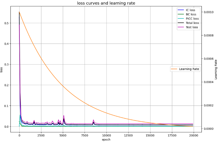
Visualization of error convergence status (Visualization 5)

# Draw loss curves

fig, ax1 = plt.subplots(figsize=(12, 8))
ax2 = ax1.twinx()

ax1.plot(Epoch, IC_loss, c='b', label='IC loss')
ax1.plot(Epoch, BC_loss, c='g', label='BC loss')
ax1.plot(Epoch, PINN_loss, c='c', label='PICC loss')
ax1.plot(Epoch, Total_loss, c='k', label='Total loss')
ax1.plot(Epoch, Test_loss, c='m', label='Test loss')
ax1.set_xlabel('epoch')
ax1.set_ylabel('loss')
ax1.set_title('loss curves and learning rate', fontsize='14')
ax1.grid()
ax1.legend(loc=1)

ax2.plot(Epoch, Learning_Rate, c='darkorange', label='Learning Rate')
ax2.set_ylabel('Learning Rate')
ax2.legend(loc=7)

plt.show()

Visualization results

The title of the code corresponds to the title of the code with “visualization n”.

FDM results (visualization 1)

FDM

State before PINNs start (Visualization 2)

Initial

Evaluate the learning model (visualization 3)

PINNs

Differences between PINNs and FDMs (Visualization 4)

PINNs-FDM

Error convergence status (visualization 5)

loss

Conclusion

Through this experience, I gained a better understanding of the behavior of PINNs. I also learned a little more about Python and PyTorch (especially Tensor, array dimension, automatic differentiation, etc.) through the difficulties I had (and got into) with coding.

I still do not understand the superiority of PINNs compared to FDM in terms of code difficulty and execution time (time required to find a solution).

I would like to try PINNs on phenomena related to my interests in astronomy (astrophysics).