Introduction
I have been trying to simulate steady state laminar flows with PINNs since the end of last year, but I was stumped by the derivation of the Navier Stokes (NS) equations of Cauchy stress tensor type. I coded PINNs with the governing equations based on the Velocity-pressure type NS equations. I got a result that looks like it, and I will summarize it in this post.
Sources
- PINN-laminar-flow - I used the paper and code posted on github here as a reference. I used the overall structure of the code and individual variables and constants as reference. I was stumped when it came to the Cauchy stress tensor in the original paper, which I did not understand.
- On Physics-Informed Deep Learning for Solving Navier-Stokes Equations - As mentioned in 1. above, I don’t know the Cauchy stress tensor, so I found this information while searching the net. After downloading and reading the paper, I found that there are two types of NS equations: Velocity-pressure (VP) form and Cauchy stress tensor (ST) form. From here, the following sources 3. and 4. were referenced.
- NSFnets (Navier-Stokes Flow nets): Physics-informed neural networks for the incompressible Navier-Stokes equations - referenced as VP form from source 2. There was also a description of vorticity-velocity (VV) here.
- [Physics-informed deep learning for incompressible laminar flows](https://www.sciencedirect.com/science/article/pii/S2095034920300350? via%3Dihub) - was referenced as ST form from source 2. This is the paper in source 1.
- [Applying Physics-Informed Neural Networks to Solve Navier-Stokes Equations for Laminar Flow around a Particle](https://www.mdpi. com/2297-8747/28/5/102) - A paper dealing with steady state laminar flow. It was helpful because it fit my direction. In particular, I found it helpful in the section where the loss function is summed, where it is weighted based on the difference in the number of sample points between the computational domain and the boundary conditions.
Physical background
Derivation of the governing equations
The equations of continuity and the NS equations (Navier Stokes Equations) are as follows $$ \frac{\partial \rho}{\partial t} +\nabla \cdot (\rho \boldsymbol{v}) =0 \tag{1} $$
$$ \rho \left( \frac{\partial \boldsymbol{v}}{\partial t} +(\boldsymbol{v}\cdot \nabla)\boldsymbol{v} \right) = -\nabla p+ \mu\Delta \boldsymbol{v} + \rho\boldsymbol{g} \tag{2} $$
where $\rho$ is the density of the fluid, $\boldsymbol{v}(\boldsymbol{r},t)$ is the velocity of the fluid, $p(\boldsymbol{r},t)$ is the pressure on the fluid, $\mu$ is the viscosity, $\boldsymbol{g}$ is the external force. The meaning of each term is as follows. The first term on the left side is the time derivative term and the second term is the advection term. The first term on the right side is the pressure term, the second term is the viscosity term (diffusion term), and the third term is the external force term.
Since we will be dealing with the steady state of an incompressible fluid, the equation of continuity and the NS equation are as follows.
$$ \nabla \cdot \boldsymbol{v} = 0 \tag{3} $$ In the NS equation (2), the time derivative term disappears when the steady state is considered, and the external force term disappears when the two dimensions without external force are considered, and by interchanging the left and right sides, we can write $$ -\nabla p + \mu \Delta \boldsymbol{v} = \rho(\boldsymbol{v}\cdot \nabla)\boldsymbol{v} \tag{4} $$ Expressing the above equations (3) and (4) using the two-dimensional coordinates $(x, y)$ and the velocity component $(u, v)$, we have $$ \frac{\partial u}{\partial x} + \frac{\partial v}{\partial y} = 0 \tag{5} $$
$$ -\frac{\partial p}{\partial x} + \mu \left(\frac{\partial^2 u}{\partial x^2}+\frac{\partial^2 u}{\partial y^2}\right) = \rho \left(u\frac{\partial u}{\partial x}+v\frac{\partial u}{\partial y}\right) \tag{6} $$
$$ -\frac{\partial p}{\partial y} + \mu \left(\frac{\partial^2 v}{\partial x^2}+\frac{\partial^2 v}{\partial y^2}\right) = \rho \left(u\frac{\partial v}{\partial x}+v\frac{\partial v}{\partial y}\right) \tag{7} $$
Equations (5), (6) and (7) above are the governing equations. Note that in equations (6) and (7), the left-hand side is shifted to the right-hand side and the form $=0$ is used as the governing equation.
Two Types of Navier Stokes Equations
For reference, the Velocity-pressure (VP) and Cauchy stress tensor (ST) types of the NS equation are summarized below. Adapted from source 2.
Velocity-pressure(VP) form
This is a familiar notation as follows. $$ \rho(\boldsymbol{u}\cdot\nabla)\boldsymbol{u} = -\nabla p + \mu\nabla^2\boldsymbol{u} \tag{8} $$
$$ \nabla \cdot \boldsymbol{u} = 0 \tag{9} $$
$$ \boldsymbol{u} = \boldsymbol{u}_{\Gamma} \qquad in , \Gamma_D \tag{10} $$
$$ \partial_n \boldsymbol{u} = 0 \qquad in , \Gamma_N \tag{11} $$
Where $\Gamma_D$ and $\Gamma_N$ denote Dirichlet boundary condition and Neumann boundary condition.
Cauchy stress tensor(ST) form
This one is expressed via $\sigma$, which is Cauchy stress tensor. I do not understand the derivation. $$ \rho(\boldsymbol{u}\cdot\nabla)\boldsymbol{u} = -\nabla \cdot \sigma \tag{12} $$
$$ \sigma = -p\boldsymbol{I}+\mu \left(\nabla\boldsymbol{u}+\nabla\boldsymbol{u}^T \right) \tag{13} $$
$$ \nabla \cdot \boldsymbol{u} = 0 \tag{14} $$
$$ \boldsymbol{u} = \boldsymbol{u}_{\Gamma} \qquad in , \Gamma_D \tag{15} $$
$$ \partial_n \boldsymbol{u} = 0 \qquad in , \Gamma_N \tag{16} $$
Code
import required packages, make sure you are using GPU
import numpy as np

import torch
import torch.nn as nn
import torch.nn.functional as F
from torch import optim
from torch.optim import lr_scheduler

import matplotlib.pyplot as plt

from pyDOE import lhs  # Latin Hypercube Sampling (LHS

# run on cuda if possible
device = 'cuda' if torch.cuda.is_available() else 'cpu'
print("Running on", device)
Define functions
# Remove points inside the cylinder from collocation points
#  Find the distance between the center of the cylinder (xc, yc) and a point,
#  and delete anything less than the cylinder radius (r).
def Remove_inCylinder(coor, xc, yc, r):
    distance = np.array([((xy[0] - xc)**2 + (xy[1]-yc)**2)**0.5 for xy in coor])
    return coor[distance > r, :]
The function above is a function to delete points inside a cylinder.
# Differentiation by pytorch
# return dy/dx
def gradients(y, x):
    return torch.autograd.grad(y,
                               x,
                               grad_outputs=torch.ones_like(y),
                               create_graph=True,
                              )[0]
The above function is a function that performs differentiation (partial differentiation) using torch’s function. It is defined as a function to improve the outlook of the next model function, net_f().
Create a fully-connected layer network class
# define u_NN class

class u_NN(nn.Module):
    def __init__(self, n_input, n_output, n_hiddens=[32,64,128,128,64,32]):
        super().__init__()
        self.activation = nn.Tanh()
        self.input_layer = nn.Linear(n_input, n_hiddens[0])
        self.hidden_layers = nn.ModuleList(
            [nn.Linear(n_hiddens[i], n_hiddens[i+1]) for i in range(len(n_hiddens)-1)]
        )
        self.output_layer = nn.Linear(n_hiddens[-1], n_output)

    def forward(self, x):
        x = self.activation(self.input_layer(x))
        for layer in self.hidden_layers:
            x = self.activation(layer(x))
        x = self.output_layer(x)
        return x

    def neural_net(self, x, y):
        inputs = torch.cat([x, y], dim=1)
        outputs = self.forward(inputs)
        u = outputs[:, 0:1]
        v = outputs[:, 1:2]
        p = outputs[:, 2:3]
        return u, v, p

    def net_f(self, x, y):
        x.requires_grad = True
        y.requires_grad = True
        u, v, p = self.neural_net(x, y)
        u_x = gradients(u, x)
        v_y = gradients(v, y)
        f1 = u_x + v_y

        p_x = gradients(p, x)
        u_y = gradients(u, y)
        u_xx = gradients(u_x, x)
        u_yy = gradients(u_y, y)
        f2 = p_x - mu*(u_xx + u_yy) + rho*(u*u_x + v*u_y)

        p_y = gradients(p, y)
        v_x = gradients(v, x)
        v_xx = gradients(v_x, x)
        v_yy = gradients(v_y, y)
        f3 = p_y - mu*(v_xx + v_yy) + rho*(u*v_x + v*v_y)

        return f1, f2, f3
Define problem domain (variables, constants)
wall_samples = 441
inlet_samples = 201
outlet_samples = 201

# define wall(floor, celling)
#   celling: (0, 0.41)-(1.1, 0.41)
#   floor: (0, 0)-(1.1, 0)

CEILING = [0.0, 0.41] + [1.1, 0.0] * lhs(2, wall_samples)
FLOOR = [0.0, 0.0] + [1.1, 0.0] * lhs(2, wall_samples)

# define inlet flow
#  u(0,y) = 4 * U_max * (H - y) * y / H^2
#    It is a (convex upward) quadratic curve
#    passing through 0 and H on the y-axis.
U_max = 1.0
INLET = [0.0, 0.0] + [0.0, 0.41] * lhs(2, inlet_samples)
y_INLET = INLET[:, 1:2]
u_INLET = 4 * U_max * y_INLET * (0.41 - y_INLET) / (0.41**2)
v_INLET = 0 * y_INLET
INLET = np.concatenate((INLET, u_INLET, v_INLET), 1)

# OUTLET
OUTLET = [1.1, 0.0] + [0.0, 0.41] * lhs(2, outlet_samples)
# Define cylinder surface
surface_samples = 251
r = 0.05
theta = [0.0] + (2*np.pi) * lhs(1, surface_samples)
x_CYLD = np.multiply(r, np.cos(theta)) + 0.2
y_CYLD = np.multiply(r, np.sin(theta)) + 0.2
CYLD = np.concatenate((x_CYLD, y_CYLD), 1)
# Put together walls (floors, ceilings, cylinder surfaces)
WALL = np.concatenate((CYLD, CEILING, FLOOR), 0)
# Define collocation point (See collocation method) for PINNs
coll_samples = 10000  # numper of collocation point
ref_samples = 1000  # number of refine point (around the cylinder)

lb = np.array([0, 0])
ub = np.array([1.1, 0.41])
XY_c = lb + (ub - lb) * lhs(2, coll_samples)
XY_c_refine = [0.1, 0.1] + [0.2, 0.2] * lhs(2, ref_samples)
XY_c = np.concatenate((XY_c, XY_c_refine), 0)
XY_c = Remove_inCylinder(XY_c, xc=0.2, yc=0.2, r=0.05)
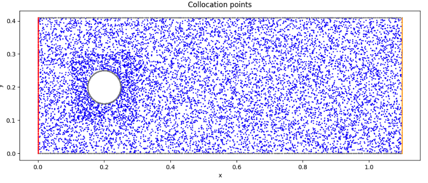
Visualize collocation points
# Visualize the collocation points
fig, ax = plt.subplots(figsize=(12,8))
ax.set_aspect('equal')
ax.scatter(XY_c[:, 0:1], XY_c[:, 1:2], marker='o', color='blue', s=1)
ax.scatter(WALL[:, 0:1], WALL[:, 1:2], marker='o', color= 'gray', s=1)
ax.scatter(OUTLET[:, 0:1], OUTLET[:, 1:2], marker='o', color='orange', s=1)
ax.scatter(INLET[:, 0:1], INLET[:, 1:2], marker='o', color='red', s=1)
ax.set_title('Collocation points')
ax.set_xlabel('x')
ax.set_ylabel('y')
plt.show()
Create a model
# Create a Model
#  Input: (x, y)
#  Output: (u, v, p)
model = u_NN(2, 3).to(device)
print(model)
Tensorize variables used for training
# Define collocation, INLET, OUTLET, and WALL variables as torch.tensor
x_c = torch.tensor(XY_c[:, 0:1], device=device, dtype=torch.float32)
y_c = torch.tensor(XY_c[:, 1:2], device=device, dtype=torch.float32)

x_INLET = torch.tensor(INLET[:, 0:1], device=device, dtype=torch.float32)
y_INLET = torch.tensor(INLET[:, 1:2], device=device, dtype=torch.float32)
u_INLET = torch.tensor(INLET[:, 2:3], device=device, dtype=torch.float32)
v_INLET = torch.tensor(INLET[:, 3:4], device=device, dtype=torch.float32)

x_OUTLET = torch.tensor(OUTLET[:, 0:1], device=device, dtype=torch.float32)
y_OUTLET = torch.tensor(OUTLET[:, 1:2], device=device, dtype=torch.float32)

x_WALL = torch.tensor(WALL[:, 0:1], device=device, dtype=torch.float32)
y_WALL = torch.tensor(WALL[:, 1:2], device=device, dtype=torch.float32)

mu = 0.02
rho = 1.0
Define loss function and optimizer function
# Loss function: Mean Square Error
loss_func = nn.MSELoss()

# Optimizer: Adam(Adaptive moment estimation)
optimizer = optim.Adam(model.parameters(), lr=0.001)

# scheduler = lr_scheduler.ExponentialLR(optimizer, gamma=0.98)
loss_func() is not used this time. Everything is handled by torch.mean().
Learning loop
# learning Loop

num_epoch = 8000  # epoch count

Epoch = []
Loss_f1 = []
Loss_f2 = []
Loss_f3 = []
Loss_f = []
Loss_t = []
Loss_WALL = []
Loss_INLET = []
Loss_OUTLET = []

for i in range(num_epoch):
    if i == 0:
        print("Epoch \t Loss_f1 \t Loss_f2 \t Loss_f3 \t Loss_f \t Loss_WALL \t Loss_INLET \t Loss_OUTLET")

    optimizer.zero_grad()
    f1, f2, f3 = model.net_f(x_c, y_c)
    loss_f1 = torch.mean(f1**2)
    loss_f2 = torch.mean(f2**2)
    loss_f3 = torch.mean(f3**2)
    loss_f = loss_f1 + loss_f2 + loss_f3

    u_wall, v_wall, _ = model.neural_net(x_WALL, y_WALL)
    loss_WALL = torch.mean(u_wall**2) + torch.mean(v_wall**2)

    u_inlet, v_inlet, _ = model.neural_net(x_INLET, y_INLET)
    loss_INLET = torch.mean((u_inlet - u_INLET)**2) + torch.mean((v_inlet - v_INLET)**2)

    _, _, p_outlet = model.neural_net(x_OUTLET, y_OUTLET)
    loss_OUTLET = torch.mean(p_outlet**2)

    loss_t = loss_f + 2*(loss_WALL + loss_INLET + loss_OUTLET)

    loss_t.backward()
    optimizer.step()

    if i % 100 == 0:
        Epoch.append(i)
        Loss_f1.append(loss_f1.detach().cpu().numpy())
        Loss_f2.append(loss_f2.detach().cpu().numpy())
        Loss_f3.append(loss_f3.detach().cpu().numpy())
        Loss_f.append(loss_f.detach().cpu().numpy())
        Loss_t.append(loss_t.detach().cpu().numpy())
        Loss_WALL.append(loss_WALL.detach().cpu().numpy())
        Loss_INLET.append(loss_INLET.detach().cpu().numpy())
        Loss_OUTLET.append(loss_OUTLET.detach().cpu().numpy())

    if i % 1000 == 0:
        print(i, "\t",
              format(loss_f1.detach().cpu().numpy(), ".4E"), "\t",
              format(loss_f2.detach().cpu().numpy(), ".4E"), "\t",
              format(loss_f3.detach().cpu().numpy(), ".4E"), "\t",
              format(loss_f.detach().cpu().numpy(), ".4E"), "\t",
              format(loss_WALL.detach().cpu().numpy(), ".4E"), "\t",
              format(loss_INLET.detach().cpu().numpy(), ".4E"), "\t",
              format(loss_OUTLET.detach().cpu().numpy(), ".4E"), "\t",
             )
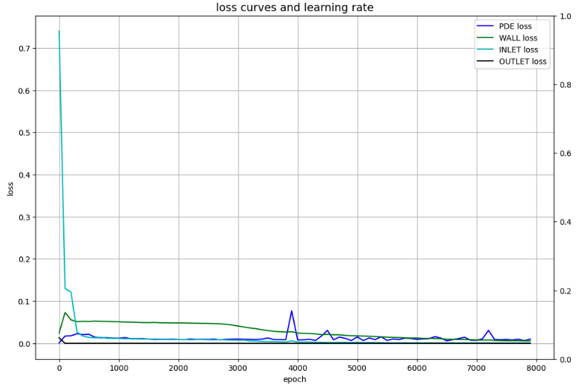
Visualize losses
# Draw loss curves

fig, ax1 = plt.subplots(figsize=(12, 8))
ax2 = ax1.twinx()

ax1.plot(Epoch, Loss_f, c='b', label='PDE loss')
ax1.plot(Epoch, Loss_WALL, c='g', label='WALL loss')
ax1.plot(Epoch, Loss_INLET, c='c', label='INLET loss')
ax1.plot(Epoch, Loss_OUTLET, c='k', label='OUTLET loss')
ax1.set_xlabel('epoch')
ax1.set_ylabel('loss')
ax1.set_title('loss curves and learning rate', fontsize='14')
ax1.grid()
ax1.legend()

plt.show()
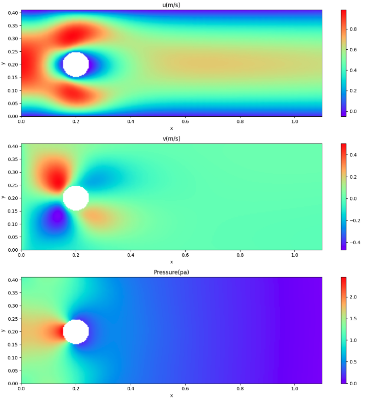
Displays velocity and pressure fields
# Using the learned model,
# find u,v,p in the form of collocation coordinates of x,y

x_collo = np.linspace(0, 1.1, 251)
y_collo = np.linspace(0, 0.41, 101)
X, Y = np.meshgrid(x_collo, y_collo)

# Remove cylinder internals
X = X.flatten()[:, None]
Y = Y.flatten()[:, None]
dst = ((X - 0.2)**2 + (Y - 0.2)**2)**0.5
X = X[dst >= 0.05]
Y = Y[dst >= 0.05]

# Convert to tensor
x_collo = torch.tensor(X.flatten()[:, None], device=device, dtype=torch.float32)
y_collo = torch.tensor(Y.flatten()[:, None], device=device, dtype=torch.float32)

# Predicts speed and pressure
u_pred, v_pred, p_pred = model.neural_net(x_collo, y_collo)

u_pred = u_pred.to("cpu").detach().numpy()
v_pred = v_pred.to("cpu").detach().numpy()
p_pred = p_pred.to("cpu").detach().numpy()
I was thinking of using contourf() to display contour lines, but when a cylinder part is hollowed out as in this case, the conversion to two dimensions does not work well, so I decided to use scatter() to display the contour lines.
# Visualize predicted velocity, pressure

alpha = 1.0
cmap = 'rainbow'
marker= 'o'
s = 20

fig = plt.figure(figsize=(12,12))
ax1 = fig.add_subplot(3, 1, 1)
cp = ax1.scatter(X, Y, c=u_pred, alpha=alpha, edgecolors='none', cmap=cmap, marker=marker, s=s)
fig.colorbar(cp)
ax1.set_xlim([0, 1.1])
ax1.set_ylim([0, 0.41])
ax1.set_title('u(m/s)')
ax1.set_xlabel('x')
ax1.set_ylabel('y')

ax2 = fig.add_subplot(3, 1, 2)
cp = ax2.scatter(X, Y, c=v_pred, alpha=alpha, edgecolors='none', cmap=cmap, marker='o', s=s)
fig.colorbar(cp)
ax2.set_xlim([0, 1.1])
ax2.set_ylim([0, 0.41])
ax2.set_title('v(m/s)')
ax2.set_xlabel('x')
ax2.set_ylabel('y')

ax3 = fig.add_subplot(3, 1, 3)
cp = ax3.scatter(X, Y, c=p_pred, alpha=alpha, edgecolors='none', cmap=cmap, marker='o', s=s)
fig.colorbar(cp)
ax3.set_xlim([0, 1.1])
ax3.set_ylim([0, 0.41])
ax3.set_title('Pressure(pa)')
ax3.set_xlabel('x')
ax3.set_ylabel('y')

plt.tight_layout()
plt.show()
Visualization results
Initial state (collocation points)

Transition of Losses

Inference results for velocity and pressure fields

Summary
The visualization of the results of inferring the region of interest by PINNs was summarized here because the results of velocity and pressure fields as seen in the information sources were obtained. Therefore, I have not been able to compare the obtained results (numerical values) with results from other methods. As one of the other methods to be compared, I’m considering OpenFoam, which I have been working on recently.
In this case, I assumed a steady state, so I did not include time as a variable. Source 1. also has a problem setup that includes time, so I would like to try that next time. Furthermore, I would like to simulate even the generation of Karman’s vortex with PINNs.