Simulation of 2D flow over cylinder

Introduction

Two months ago in this post, laminar flow around a 2D circular cylinder (Laminar Flow), using the governing equations for each of the ST and VP forms, The simulation was performed using the governing equations for each of the ST form and VP form.

Since then, we have simulated the flow around a 2-D cylinder in the time range 0 to 60 seconds for various parameters, and the results are summarized here.

Sources

Physics-Informed Neural Networks for Low Reynolds Number Flows over Cylinder - I proceeded by referring to the computational domain of this paper. The description of the wall boundary condition was “the freestream baoundary condition of 1 m/s” in the description of Figure 4. The description of the number of hidden layers was also helpful, along with the figure in Figure 9. There is no source code, but from the description of the governing equations of the fluid, it seems to be solved in VP type. the Input of the overall picture in Figure 2. has a description of time $t$, but no time axis.
Experience report of physics-informed neural networks in fluid simulations: pitfalls and frustration - I referred to this paper for the boundary conditions, the number of nodes in the hidden layer, and the number of layers (layers). Note that this paper was written about a year before that paper, by the same author as source 1. of Kalman Vortex with OpenFOAM, which I posted a while ago.
Vortex shedding by Joel Guerrero 2D - The tutorial “2D Circular cylinder - Vortex shedding” can be found on this page. Initially, the simulation was done in PINNs to match the computational domain of this tutorial. This page is introduced in the source 6. of the contribution with Kalman vortex with OpenFOAM.
Summary of PINN Devices - Links to resources that can give you tips on what to do if your learning is not going well with PINN. Using this as a starting point, I did a lot of research on “failure mode”.

Background

The parameters were changed according to the following process. The results should be judged by looking at the time history of the velocity field/pressure field, and judging the natural one with sensitivity, and comparing it with the output of OpenFOAM, etc. However, I could not go that far this time.

1. Change of calculation domain

At first, in order to compare simulation results, I started with the computational domain of the tutorial in source 6. of OpenFOAM. No good results were obtained, and once to check for errors in the code, the simulation was conducted in the computation domain in this post. As a result, I decided to run the simulation in ST form since the results were better in ST form.

For the computational domain, the back of the cylinder was lengthened in accordance with Source 1. In the case of U_max=5 (Re=200), relatively good results were obtained for the velocity field, but the pressure field was skewed in the y direction. ), both the velocity and pressure fields were significantly disturbed.

For the upper and lower walls, the slip condition (U_max value in the u direction and zero in the v direction) gave relatively good results for both the velocity and pressure fields.

2. change hidden layer (increase hidden layer)

The simulation results in ST form showed relatively good results for the u and v velocity components, but I was concerned about the extension to the front of the cylinder (INLET side) (I call this the nose), so I looked into it and found that in the explanation of Figure 9. in Source 1., “When the hidden layer is 10, the tip is not accurately reproduced and the description was “The tip cannot be accurately reproduced when the number of hidden layers is 10. I decided to increase the number of hidden layers.

3. Response to the lack of convergence

The hidden layer was implemented with 50 nodes x 13 layers, but it was implemented with 50 nodes x 20 layers and 25 layers. Then, even after 20,000 loops (epoch=20,000), the error both INLET and WALL did not move from 1.0, and the phenomenon did not converge.

Referring to the information source 4., I tried various countermeasures such as weighting the error (loss term), initializing the network with “xavier,” and so on.

As a result, when the model was run with 50 nodes x 25 hidden layers and epoch=50,000, the error both INLET and WALL decreased drastically from 1.0 after 20,000 times, showing a convergence trend. The results inferred from the model were different from what was expected for both the velocity and pressure fields. In particular, the velocity field was tilted in the u-direction, whereas it was originally tilted in the v-direction.

4. Change the hidden layer (increase the number of nodes)

Since I could not obtain very good results with 50 nodes, we tried 256 nodes/512 nodes x 6 layers/8 layers, referring to Source 2. Finally, 256 nodes x 8 layers gave the best results.

Parameters

As described in the background, the hidden layer, boundary conditions, collocation point, number of iterations (epoch), etc. were changed in various ways, but in the following code, simulations were performed with the following parameter settings.

For the collocation point, please refer to the code in the “Setting the problem domain (variables and constants)” section.

Parameters	Contents
hidden layers	256ｘ256 node8 layers
INLET	1.0 （U_max=1.0m/s flow in x direction）
WALL（upper and lower boundaries）	slip condition（U_max flow in x direction）
OUTLET	pressure zero
epoch	100,000 times

Code

Some parts are the same as in this post, but I will post the code again.

import package

import os
import numpy as np

import torch
import torch.nn as nn
import torch.nn.functional as F
from torch import optim
from torch.optim import lr_scheduler

import matplotlib.pyplot as plt
from matplotlib.colors import Normalize

from pyDOE import lhs  # Latin Hypercube Sampling (LHS)

import subprocess

Confirmation that we are using CUDA

# Exit if not run on cuda
if not torch.cuda.is_available():
    print("Exit because of running on cpu\n")
    os._exit(os.EX_OK)
else:
    device = 'cuda'  # device is used later

# We are running on cuda
cmd = "nvidia-smi --query-gpu=name --format=csv,noheader"
output = subprocess.check_output(cmd, shell=True).decode()
output = output.replace("\n", "")
print("Running on", output)

In rare cases, CUDA is not recognized and the CPU is used for execution. So, if CUDA was not found, we would stop execution.

Define function

# Remove points inside the cylinder from collocation points
#  Find the distance between the center of the cylinder (xc, yc) and a point,
#  and delete anything less than the cylinder radius (r).
def Remove_inCylinder(coor, xc, yc, r):
    distance = np.array([((xy[0] - xc)**2 + (xy[1]-yc)**2)**0.5 for xy in coor])
    return coor[distance > r, :]

Define Reynolds number

# Define Re

U_max = 1.0 # flow velocity
mu = 0.0005
rho = 1.0  # Re=200=(uxD)/nu=(1x0.1)/0.0005, nu=mu/rho

Define problem domain (variables, constants)

# Define variables to represent computation domains

# Some constants
IC_samples = 5000
wall_samples = 1000
cylinder_samples = 5000
inlet_samples = 2000
outlet_samples = 2000

# Domain bounds
xmin = 0.0
ymin = 0.0
tmin = 0.0
xmax = 4.0
ymax = 2.0
tmax = 60.0
lb = np.array([xmin, ymin, tmin])
ub = np.array([xmax, ymax, tmax])

# cylinder
dia = 0.1  # diameter
radi = dia/2.0  # radius
xcent = 1.0  # center in x-axis
ycent = 1.0  # cneter in y-axis

# constants for refinement area and near wall area
xrefmin = 0.5
yrefmin = 0.5
xrefmax = 3.5
yrefmax = 1.5
near_w = 0.2

# Inital Condition: 
#  (u, v, p) = (0, 0, 0)　at t= 0, x ∈ [xmin, xmax], y ∈ [ymin, ymax]

xy_IC = [xmin, ymin] + [xmax, ymax] * lhs(2, IC_samples)
t_IC = np.zeros((IC_samples, 1))
IC = np.concatenate((xy_IC, t_IC), 1)
IC = Remove_inCylinder(IC, xc=xcent, yc=ycent, r=radi)

# define floor and ceiling, we called wall
#   celling(x,y,t): (xmin, ymin ,tmin)-(xmax, ymax, tmax)
#   floor(x,y,t): (xmin, ymin, tmin)-(xmax, ymin, tmax)
# N.B. we give the constant flow at the wall.
CEILING = [xmin, ymax, tmin] + [xmax, ymin, tmax] * lhs(3, wall_samples)
x_CEILING = CEILING[:, 0:1]
u_CEILING = np.zeros_like(x_CEILING)
u_CEILING.fill(U_max)
v_CEILING = 0 * u_CEILING
CEILING = np.concatenate((CEILING, u_CEILING, v_CEILING), 1)
FLOOR = [xmin, ymin, tmin] + [xmax, ymin, tmax] * lhs(3, wall_samples)
x_FLOOR = FLOOR[:, 0:1]
u_FLOOR = np.zeros_like(x_FLOOR)
u_FLOOR.fill(U_max)
v_FLOOR = 0 * u_FLOOR
FLOOR = np.concatenate((FLOOR, u_FLOOR, v_FLOOR), 1)
WALL = np.concatenate((CEILING, FLOOR), 0)

# Define cylinder surface
rt_CYLD = [0.0, tmin] + [2*np.pi, tmax] * lhs(2, cylinder_samples)
x_CYLD = np.multiply(radi, np.cos(rt_CYLD[:, 0:1])) + xcent
y_CYLD = np.multiply(radi, np.sin(rt_CYLD[:, 0:1])) + ycent
CYLD = np.concatenate((x_CYLD, y_CYLD, rt_CYLD[:, 1:2]), 1)

# Define INLET
INLET = [xmin, ymin, tmin] + [xmin, ymax, tmax] * lhs(3, inlet_samples)
y_INLET = INLET[:, 1:2]
t_INLET = INLET[:, 2:3]
u_INLET = np.zeros_like(y_INLET)
u_INLET.fill(U_max)
v_INLET = np.zeros_like(u_INLET)
INLET = np.concatenate((INLET, u_INLET, v_INLET), 1)

# Define OUTLET
OUTLET = [xmax, ymin, tmin] + [xmin, ymax, tmax] * lhs(3, outlet_samples)

# Define Collocation points, with refinement near the wall
collo_samples = 10000
refine_samples = 5000
near_samples = 2000

"""
xyt_Collo = lb + (ub - lb) * lhs(3, collo_samples)
xyt_refine = [xrefmin, yrefmin, tmin] + [xrefmax-xrefmin, yrefmax-xrefmin, tmax] * lhs(3, refine_samples)
xyt_floor = [xmin, ymin, tmin] + [xmax, near_w, tmax] * lhs(3, near_samples)
xyt_ceiling = [xmin, ymax-near_w, tmin] + [xmax, near_w, tmax] * lhs(3, near_samples)
Collo = np.concatenate((xyt_Collo, xyt_refine, xyt_floor, xyt_ceiling), 0)
"""
collo_samples = 20000
Collo = lb + (ub - lb) * lhs(3, collo_samples)
Collo = Remove_inCylinder(Collo, xc=xcent, yc=ycent, r=radi)

In the calculation area (collocation), the effect of the points around the cylinder and around the wall was questionable, so it was removed.

Visualize collocation points

# Visualize the collocation points in (x, y, t）
fig = plt.figure(figsize=(20,20))

# 2D
ax1 = fig.add_subplot(2, 1, 1)
ax1.set_aspect('equal')
ax1.scatter(Collo[:, 0:1], Collo[:, 1:2], marker='o', color='greenyellow', s=1)
ax1.scatter(IC[:, 0:1], IC[:, 1:2], marker='o', color='magenta', s=1)
ax1.scatter(WALL[:, 0:1], WALL[:, 1:2], marker='o', color= 'orange', s=1)
ax1.scatter(CYLD[:, 0:1], CYLD[:, 1:2], marker='o', color='blue', s=1)
ax1.scatter(OUTLET[:, 0:1], OUTLET[:, 1:2], marker='o', color='gray', s=1)
ax1.scatter(INLET[:, 0:1], INLET[:, 1:2], marker='o', color='red', s=1)
ax1.set_title('Collocation points')
ax1.set_xlabel('x')
ax1.set_ylabel('y')

# 3D
ax2 = fig.add_subplot(2, 1, 2, projection='3d')
#ax2.set_aspect('equal')
ax2.set_box_aspect((2, 2, 1))
ax2.scatter(Collo[:, 0:1], Collo[:, 2:3], Collo[:, 1:2], marker='o', color='greenyellow', s=1)
ax2.scatter(WALL[:, 0:1], WALL[:, 2:3], WALL[:, 1:2], marker='o', color= 'orange', s=1)
ax2.scatter(CYLD[:, 0:1], CYLD[:, 2:3], CYLD[:, 1:2], marker='o', color='blue', s=1)
ax2.scatter(OUTLET[:, 0:1], OUTLET[:, 2:3], OUTLET[:, 1:2], marker='o', color='gray', s=1)
ax2.scatter(INLET[:, 0:1], INLET[:, 2:3], INLET[:, 1:2], marker='o', color='red', s=1)
ax2.set_title('Collocation points')
ax2.set_xlabel('x')
ax2.set_zlabel('y')
ax2.set_ylabel('t')

plt.show()

Tensorize variables used for training

# Define collocation, INLET, OUTLET, and WALL variables as torch.tensor
x_c = torch.tensor(Collo[:, 0:1], device=device, dtype=torch.float32)
y_c = torch.tensor(Collo[:, 1:2], device=device, dtype=torch.float32)
t_c = torch.tensor(Collo[:, 2:3], device=device, dtype=torch.float32)

x_IC = torch.tensor(IC[:, 0:1], device=device, dtype=torch.float32)
y_IC = torch.tensor(IC[:, 1:2], device=device, dtype=torch.float32)
t_IC = torch.tensor(IC[:, 2:3], device=device, dtype=torch.float32)

x_INLET = torch.tensor(INLET[:, 0:1], device=device, dtype=torch.float32)
y_INLET = torch.tensor(INLET[:, 1:2], device=device, dtype=torch.float32)
t_INLET = torch.tensor(INLET[:, 2:3], device=device, dtype=torch.float32)
u_INLET = torch.tensor(INLET[:, 3:4], device=device, dtype=torch.float32)
v_INLET = torch.tensor(INLET[:, 4:5], device=device, dtype=torch.float32)

x_OUTLET = torch.tensor(OUTLET[:, 0:1], device=device, dtype=torch.float32)
y_OUTLET = torch.tensor(OUTLET[:, 1:2], device=device, dtype=torch.float32)
t_OUTLET = torch.tensor(OUTLET[:, 2:3], device=device, dtype=torch.float32)


x_WALL = torch.tensor(WALL[:, 0:1], device=device, dtype=torch.float32)
y_WALL = torch.tensor(WALL[:, 1:2], device=device, dtype=torch.float32)
t_WALL = torch.tensor(WALL[:, 2:3], device=device, dtype=torch.float32)
u_WALL = torch.tensor(WALL[:, 3:4], device=device, dtype=torch.float32)
v_WALL = torch.tensor(WALL[:, 4:5], device=device, dtype=torch.float32)

x_CYLD = torch.tensor(CYLD[:, 0:1], device=device, dtype=torch.float32)
y_CYLD = torch.tensor(CYLD[:, 1:2], device=device, dtype=torch.float32)
t_CYLD = torch.tensor(CYLD[:, 2:3], device=device, dtype=torch.float32)

Create a fully-connected layer network class

# define p_NN class

class p_NN(nn.Module):
    def __init__(self, layers):
        super().__init__()
        self.activation = nn.Tanh()
#        self.activation = nn.ReLU()        
        self.input_layer = nn.Linear(layers[0], layers[1])
        self.hidden_layers = nn.ModuleList(
            [nn.Linear(layers[i], layers[i+1]) for i in range(1, len(layers)-2)]
        )
        self.output_layer = nn.Linear(layers[-2], layers[-1])
        """
        # xavier initialization
        for i in range(len(self.hidden_layers)):
            nn.init.xavier_normal_(self.hidden_layers[i].weight.data, gain=1.0)
            nn.init.zeros_(self.hidden_layers[i].bias.data)
        """

    def forward(self, x):
        x = self.activation(self.input_layer(x))
        for layer in self.hidden_layers:
            x = self.activation(layer(x))
        x = self.output_layer(x)
        return x

    def neural_net(self, x, y, t):
        inputs = torch.cat([x, y, t], dim=1)
        outputs = self.forward(inputs)
        psi = outputs[:, 0:1]
        p = outputs[:, 1:2]
        s11 = outputs[:, 2:3]
        s22 = outputs[:, 3:4]
        s12 = outputs[:, 4:5]

        return psi, p, s11, s22, s12

    def net_uvp(self, x, y, t):
        x.requires_grad = True
        y.requires_grad = True
        t.requires_grad = True
        psi, p, s11, s22, s12 = self.neural_net(x, y, t)
        u = gradients(psi, y)
        v = -gradients(psi, x)

        return u, v, p, s11, s22, s12
     
    def net_f(self, x, y, t):
        u, v, p, s11, s22, s12 = self.net_uvp(x, y, t)       
        u_x = gradients(u, x)
        u_y = gradients(u, y)
        u_t = gradients(u, t)
        s11_x = gradients(s11, x)
        s12_y = gradients(s12, y)
        fu = rho*u_t + rho*(u*u_x + v*u_y) - (s11_x + s12_y)

        v_x = gradients(v, x)
        v_y = gradients(v, y)
        v_t = gradients(v, t)
        s12_x = gradients(s12, x)
        s22_y = gradients(s22, y)
        fv = rho*v_t + rho*(u*v_x + v*v_y) - (s12_x + s22_y)

        fxx = -p + mu*2.0*u_x - s11
        fyy = -p + mu*2.0*v_y - s22
        fxy = mu*(u_y + v_x) - s12
        fp = p + (s11 + s22)/2.0

        return fu, fv, fxx, fyy, fxy, fp

    def predict(self, x, y, t):  # no tensor is passed, return no tensor
        xx = torch.tensor(x, device=device, dtype=torch.float32)
        yy = torch.tensor(y, device=device, dtype=torch.float32)
        tt = torch.tensor(t, device=device, dtype=torch.float32)
        uu, vv, pp, _, _, _ = self.net_uvp(xx, yy, tt)
        u = uu.to("cpu").detach().numpy()
        v = vv.to("cpu").detach().numpy()
        p = pp.to("cpu").detach().numpy()
        return u, v, p

I tried to initialize the network with xavier, but it didn’t work, so I commented it out.

Define differential function

# Differentiation by pytorch
# return dy/dx
def gradients(y, x):
    return torch.autograd.grad(y,
                               x,
                               grad_outputs=torch.ones_like(y),
                               create_graph=True,
                              )[0]

Create a model（Instantiate）

# Create a Model
#  Input: (x, y, t)
#  hidden: 20-layer　ｘ　50-node
#  Output: (phi, p, s1, s2, s3)
#uv_layers = [3]+20*[50]+[5]
#uv_layers = [3]+13*[50]+[5]
#uv_layers = [3]+14*[50]+[5]
#uv_layers = [3]+15*[50]+[5]
#uv_layers = [3]+10*[50]+[5]
#uv_layers = [3]+[32]+[64]+[128]+[128]+[64]+[32]+[5]
#uv_layers = [3]+[32]+[64]+[128]+[256]+[256]+[128]+[64]+[32]+[5]
#uv_layers = [3]+15*[60]+[5]

uv_layers = [3]+8*[256]+[5]

model = p_NN(uv_layers).to(device)
print(model)

Define loss function and optimizer function

# Loss function: Mean Square Error
loss_func = nn.MSELoss()

# Optimizer: Adam(Adaptive moment estimation)
optimizer = optim.Adam(model.parameters(), lr=0.005)

scheduler = lr_scheduler.ExponentialLR(optimizer, gamma=0.98)

As before, loss_func() is not used. Added a function to vary the learning rate.

Start timer to measure the time of the learning loop

#　Measure processing time

import time

start_time = time.time()

Learning loop

# learning Loop

Lamb_iw = 1.0
Lamb_ot = 1.0

num_epoch = 100000  # epoch count

Epoch = []
Learning_rate = []
Loss_fv = []
Loss_fu = []
Loss_fxx = []
Loss_fyy = []
Loss_fxy = []
Loss_fp = []
Loss_PINN = []
Loss_TOTAL = []
Loss_IC = []
Loss_WALL = []
Loss_CYLD = []
Loss_INLET = []
Loss_OUTLET = []

for i in range(num_epoch):
    if i == 0:
        print("Epoch \t Learning-rate \t Loss_Total \t Loss_PINN \t Loss_IC \t Loss_WALL \t Loss_CYLD \t Loss_INLET \t Loss_OUTLET")

    optimizer.zero_grad()
    fu, fv, fxx, fyy, fxy, fp = model.net_f(x_c, y_c, t_c)
    loss_fu = torch.mean(fu**2)
    loss_fv = torch.mean(fv**2)
    loss_fxx = torch.mean(fxx**2)
    loss_fyy = torch.mean(fyy**2)
    loss_fxy = torch.mean(fxy**2)
    loss_fp = torch.mean(fp**2)
    loss_PINN = loss_fu + loss_fv + loss_fxx + loss_fyy + loss_fxy + loss_fp
    
    u_ic, v_ic, p_ic, _, _, _ = model.net_uvp(x_IC, y_IC, t_IC)
    loss_IC = torch.mean(u_ic**2) + torch.mean(v_ic**2) + torch.mean(p_ic**2)
    
    u_wall, v_wall, _, _, _, _ = model.net_uvp(x_WALL, y_WALL, t_WALL)
#    loss_WALL = torch.mean(u_wall**2) + torch.mean(v_wall**2)
    loss_WALL = torch.mean((u_wall - u_WALL)**2) + torch.mean((v_wall - v_WALL)**2)

    u_cyld, v_cyld, _, _, _, _ = model.net_uvp(x_CYLD, y_CYLD, t_CYLD)
    loss_CYLD = torch.mean(u_cyld**2) + torch.mean(v_cyld**2)
    
    u_inlet, v_inlet, _, _, _, _ = model.net_uvp(x_INLET, y_INLET, t_INLET)
    loss_INLET = torch.mean((u_inlet - u_INLET)**2) + torch.mean(v_inlet**2)
    
    _, _, p_outlet, _, _, _ = model.net_uvp(x_OUTLET, y_OUTLET, t_OUTLET)
    loss_OUTLET = torch.mean(p_outlet**2)
    # Apply zero-gradient condition at OUTLET
#    x_OUTLET.requres_grad = True
#    y_OUTLET.requres_grad = True
#    u_outlet, v_outlet, _, _, _, _ = model.net_uvp(x_OUTLET, y_OUTLET, t_OUTLET)
#    u_outlet_x = gradients(u_outlet, x_OUTLET)
#    v_outlet_x = gradients(v_outlet, x_OUTLET)
#    loss_OUTLET = torch.mean(u_outlet_x**2) + torch.mean(v_outlet_x**2)

    loss_TOTAL = (loss_PINN + loss_IC + loss_CYLD + loss_OUTLET) * Lamb_ot + (loss_WALL + loss_INLET) * Lamb_iw

    loss_TOTAL.backward()
    optimizer.step()

    if i % 100 == 0:
        Epoch.append(i)
        Learning_rate.append(scheduler.get_last_lr()[0])
        Loss_fu.append(loss_fu.detach().cpu().numpy())
        Loss_fv.append(loss_fv.detach().cpu().numpy())
        Loss_fxx.append(loss_fxx.detach().cpu().numpy())
        Loss_fyy.append(loss_fyy.detach().cpu().numpy())
        Loss_fxy.append(loss_fxy.detach().cpu().numpy())
        Loss_fp.append(loss_fp.detach().cpu().numpy())
        Loss_PINN.append(loss_PINN.detach().cpu().numpy())
        Loss_TOTAL.append(loss_TOTAL.detach().cpu().numpy())
        Loss_IC.append(loss_IC.detach().cpu().numpy())
        Loss_WALL.append(loss_WALL.detach().cpu().numpy())
        Loss_CYLD.append(loss_CYLD.detach().cpu().numpy())
        Loss_INLET.append(loss_INLET.detach().cpu().numpy())
        Loss_OUTLET.append(loss_OUTLET.detach().cpu().numpy())

        scheduler.step()

    if i % 1000 == 0:
        print(i, "\t",
              format(scheduler.get_last_lr()[0], ".4E"), "\t",
              format(loss_TOTAL.detach().cpu().numpy(), ".4E"), "\t",
              format(loss_PINN.detach().cpu().numpy(), ".4E"), "\t",
              format(loss_IC.detach().cpu().numpy(), ".4E"), "\t",
              format(loss_WALL.detach().cpu().numpy(), ".4E"), "\t",
              format(loss_CYLD.detach().cpu().numpy(), ".4E"), "\t",
              format(loss_INLET.detach().cpu().numpy(), ".4E"), "\t",
              format(loss_OUTLET.detach().cpu().numpy(), ".4E"), "\t",
             )

Comment out the non-slip condition on the wall and the zero velocity gradient at OUTLET.

Timer is stopped because the learning loop has ended.

end_time = time.time()
processing_time = end_time - start_time
print("#"*20)
print("processing_time(sec): ", processing_time)
print("#"*20)

Visualize losses

# Draw loss curves

fig, ax1 = plt.subplots(figsize=(12, 8))
ax2 = ax1.twinx()

ax1.plot(Epoch, Loss_TOTAL, c='black', label='Total loss')
ax1.plot(Epoch, Loss_PINN, c='red', label='PINN loss')
ax1.plot(Epoch, Loss_IC, c='b', label='IC loss')
ax1.plot(Epoch, Loss_WALL, c='g', label='WALL loss')
ax1.plot(Epoch, Loss_INLET, c='c', label='INLET loss')
ax1.plot(Epoch, Loss_OUTLET, c='m', label='OUTLET loss')
ax1.set_xlabel('epoch')
ax1.set_ylabel('loss')
ax1.set_ylim([0, 2.0])
ax1.set_title('loss curves and learning rate', fontsize='14')
ax1.grid()
ax1.legend(loc=1)

ax2.plot(Epoch, Learning_rate, c='darkorange', label='Learning Rate')
ax2.set_ylabel('Learning Rate')
ax2.legend(loc=7)

plt.show()

Visulalize velocity and pressure fields

# File output function

alpha = 1.0
cmap = 'rainbow'
marker= 'o'
s = 20

def make_aFrame(epoch, t, x, y, u, v, p):
    """
    i: frame number: 0-100
    x, y: 2d computational domain
    u, v, p: predicted u, v, p
    """
    fig = plt.figure(figsize=(12,14))
    ax1 = fig.add_subplot(3, 1, 1)
#    norm = Normalize(vmin=0, vmax=1.2)
#    cp = ax1.scatter(x, y, c=u, alpha=alpha, edgecolors='none', cmap=cmap, marker=marker, s=s, norm=norm)
    cp = ax1.scatter(x, y, c=u, alpha=alpha, edgecolors='none', cmap=cmap, marker=marker, s=s)
    fig.colorbar(cp)
    ax1.set_xlim([xmin, xmax])
    ax1.set_ylim([ymin, ymax])
    ax1.set_title('u(m/s)  at {:07.03f}s'.format(t))
    ax1.set_xlabel('x')
    ax1.set_ylabel('y')
    ax1.set_aspect('equal')

#    norm = Normalize(vmin=-0.6, vmax=0.6)
    ax2 = fig.add_subplot(3, 1, 2)
#    cp = ax2.scatter(x, y, c=v, alpha=alpha, edgecolors='none', cmap=cmap, marker='o', s=s, norm=norm)
    cp = ax2.scatter(x, y, c=v, alpha=alpha, edgecolors='none', cmap=cmap, marker='o', s=s)
    fig.colorbar(cp)
    ax2.set_xlim([xmin, xmax])
    ax2.set_ylim([ymin, ymax])
    ax2.set_title('v(m/s)  at {:07.03f}s'.format(t))
    ax2.set_xlabel('x')
    ax2.set_ylabel('y')
    ax2.set_aspect('equal')

#    norm = Normalize(vmin=0, vmax=2.5)
    ax3 = fig.add_subplot(3, 1, 3)
#    cp = ax3.scatter(x, y, c=p, alpha=alpha, edgecolors='none', cmap=cmap, marker='o', s=s, norm=norm)
    cp = ax3.scatter(x, y, c=p, alpha=alpha, edgecolors='none', cmap=cmap, marker='o', s=s)
    fig.colorbar(cp)
    ax3.set_xlim([xmin, xmax])
    ax3.set_ylim([ymin, ymax])
    ax3.set_title('Pressure(pa)  at {:07.03f}s'.format(t))
    ax3.set_xlabel('x')
    ax3.set_ylabel('y')
    ax3.set_aspect('equal')

    plt.suptitle('Speed and Pressure field at Epoch:{:06} Time:{:07.03f}s'.format(epoch, t), fontsize=16)
    
    plt.tight_layout
    
    fig.savefig('./output/uvp_{:06}_{:07.03f}.png'.format(epoch,t), dpi=100)
    plt.close(fig)

def output_uvp(epoch):
    # Output u, v, p at each time step
    x_collo = np.linspace(xmin, xmax, 500)
    y_collo = np.linspace(ymin, ymax, 400)
    x_collo, y_collo = np.meshgrid(x_collo, y_collo)
    x_collo = x_collo.flatten()[:, None]
    y_collo = y_collo.flatten()[:, None]

    # Remove cylinder internals
    dst = ((x_collo - xcent)**2 + (y_collo - ycent)**2)**0.5
    x_collo = x_collo[dst >= radi].flatten()[:, None]
    y_collo = y_collo[dst >= radi].flatten()[:, None]

    x_collo = x_collo.flatten()[:, None]
    y_collo = y_collo.flatten()[:, None]
    t_collo = np.zeros((x_collo.size, 1))

    # Time step loop
    count = 0
    for tt in np.arange(tmin, tmax+(tmax-tmin)/100, (tmax-tmin)/100):
        if count%2 == 0:
            t_collo.fill(tt)
            u_pred, v_pred, p_pred = model.predict(x_collo, y_collo, t_collo)
            make_aFrame(epoch, tt, x_collo, y_collo, u_pred, v_pred, p_pred)
        count += 1

Visualize the pressure at three points around a cylinder

def output_pressures(epoch):
    # Predict the time evolution of pressure 
    # at the pressure measurement point (virtual pressure probe)
    t_probe = np.linspace(tmin, tmax, 100)
    x1 = np.zeros_like(t_probe)
    x2 = np.zeros_like(t_probe)
    x3 = np.zeros_like(t_probe)
    x1.fill(xcent-radi)
    x2.fill(xcent)
    x3.fill(xcent+radi)
    y1 = np.zeros_like(t_probe)
    y2 = np.zeros_like(t_probe)
    y3 = np.zeros_like(t_probe)
    y1.fill(ycent)
    y2.fill(ycent+radi)
    y3.fill(ycent)
    x1 = x1.flatten()[:, None]
    x2 = x2.flatten()[:, None]
    x3 = x3.flatten()[:, None]
    y1 = y1.flatten()[:, None]
    y2 = y2.flatten()[:, None]
    y3 = y3.flatten()[:, None]
    t_probe = t_probe.flatten()[:, None]

    _, _, p1 = model.predict(x1, y1, t_probe)
    _, _, p2 = model.predict(x2, y2, t_probe)
    _, _, p3 = model.predict(x3, y3, t_probe)

    fig = plt.figure(figsize=(12,4))

    ax1 = fig.add_subplot(1, 3, 1)
    ax1.plot(t_probe, p1, c='b', label='at P1(front-end of cylinder)')
#    ax1.set_ylim([-0.5, 2.5])
    ax1.set_xlabel('Time(s)')
    ax1.set_ylabel('Pressure(Pa)')
    ax1.grid()
    ax1.legend()

    ax2 = fig.add_subplot(1, 3, 2)
    ax2.plot(t_probe, p2, c='b', label='at P2(upper-end of cylinder)') 
#    ax2.set_ylim([-0.5, 2.5])
    ax2.set_xlabel('Time(s)')
    ax2.set_ylabel('Pressure(Pa)')
    ax2.grid()
    ax2.legend()

    ax3 = fig.add_subplot(1, 3, 3)
    ax3.plot(t_probe, p3, c='b', label='at P3(back-end of cylinder)')
#    ax3.set_ylim([-0.5, 2.5])
    ax3.set_xlabel('Time(s)')
    ax3.set_ylabel('Pressure(Pa)')
    ax3.grid()
    ax3.legend()

    fig.suptitle('Pressure time histories at Epoch:{:06}'.format(epoch))
    plt.tight_layout

    fig.savefig('./output/pressure_{:06}.png'.format(epoch), dpi=100)
    plt.close(fig)

可視化関数を呼び出す

# output the currnet state of p_NET()
os.makedirs('./output')
output_pressures(num_epoch)
output_uvp(num_epoch)

Visualize

Loss cureves

LossCurve

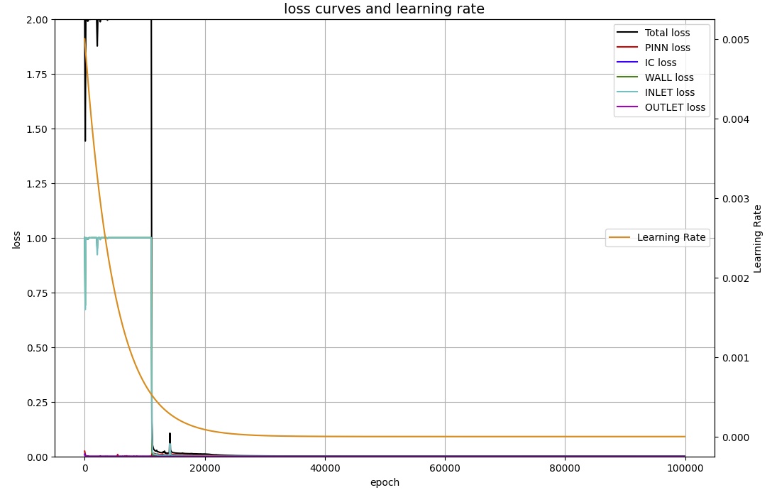
上のグラフからも分かるように、4000から11000エポックまで、WALLとINLETの誤差が1.0に留まったままとなっている。この現象は、隠れ層が深くなると（例えば50ノード・25層で）、20000エポックを過ぎても収束傾向が見られなかった。

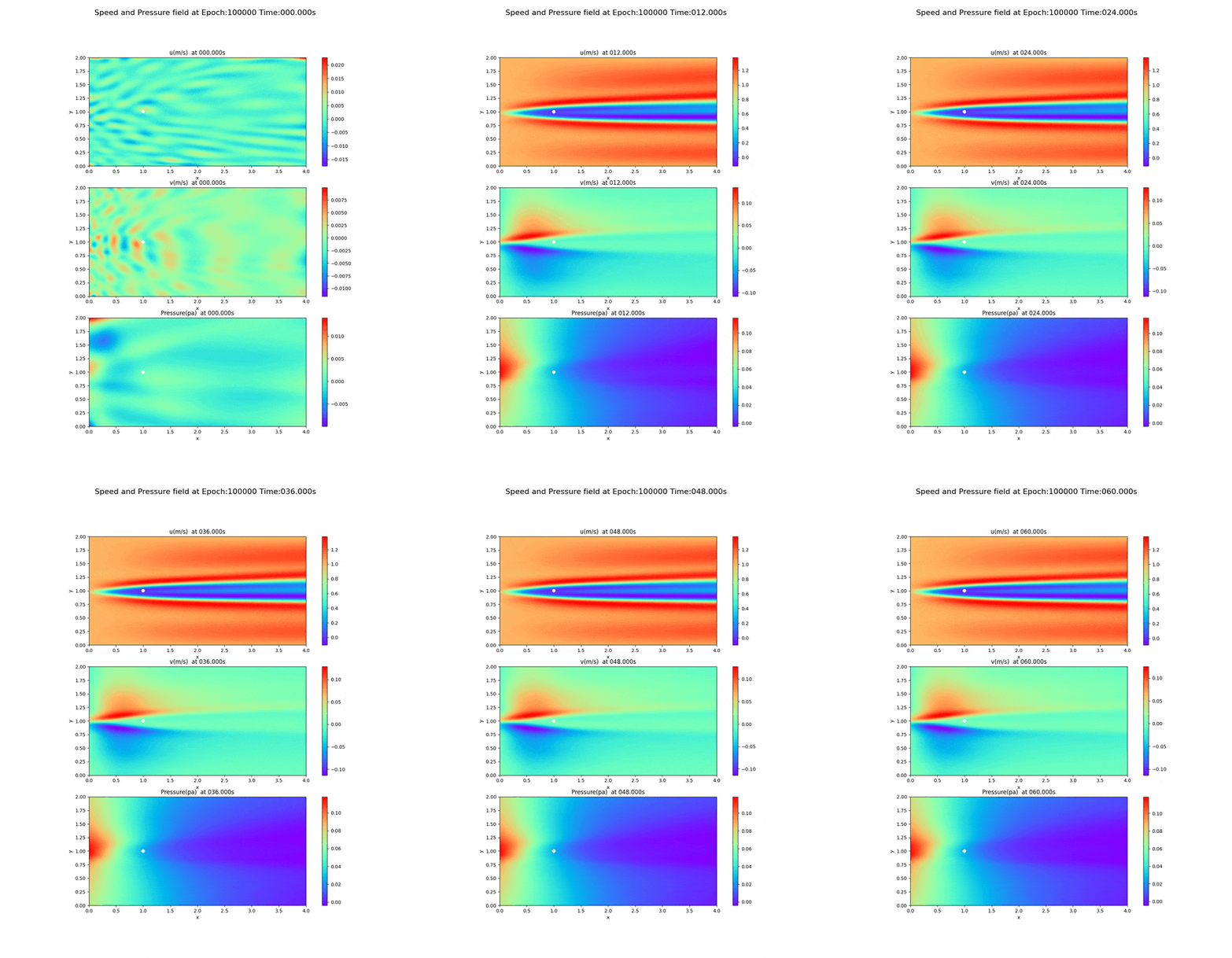
Velocity and pressure fields after 100,000 epoch

This is a movie (gif file) of the png files of the velocity and pressure fields run at epoch=100000. (The original file was 13.8 MB, so it was compressed to a smaller size.)

uvp_resize_compress

Velocity and pressure fields of less than 100,000 epoch

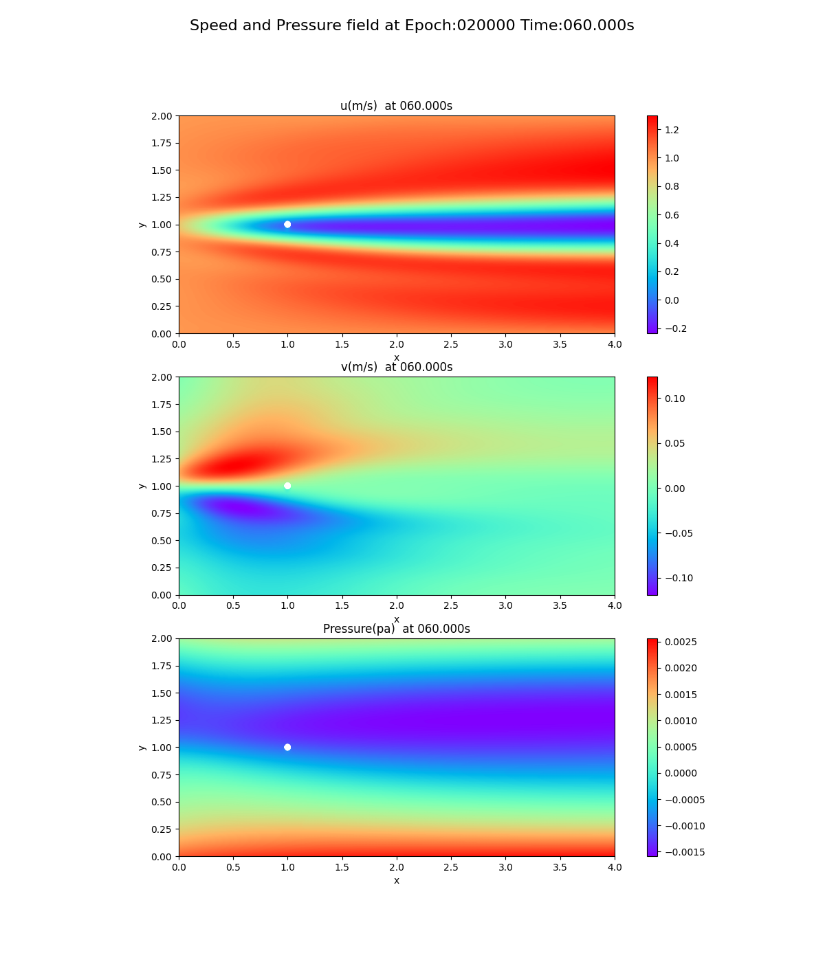
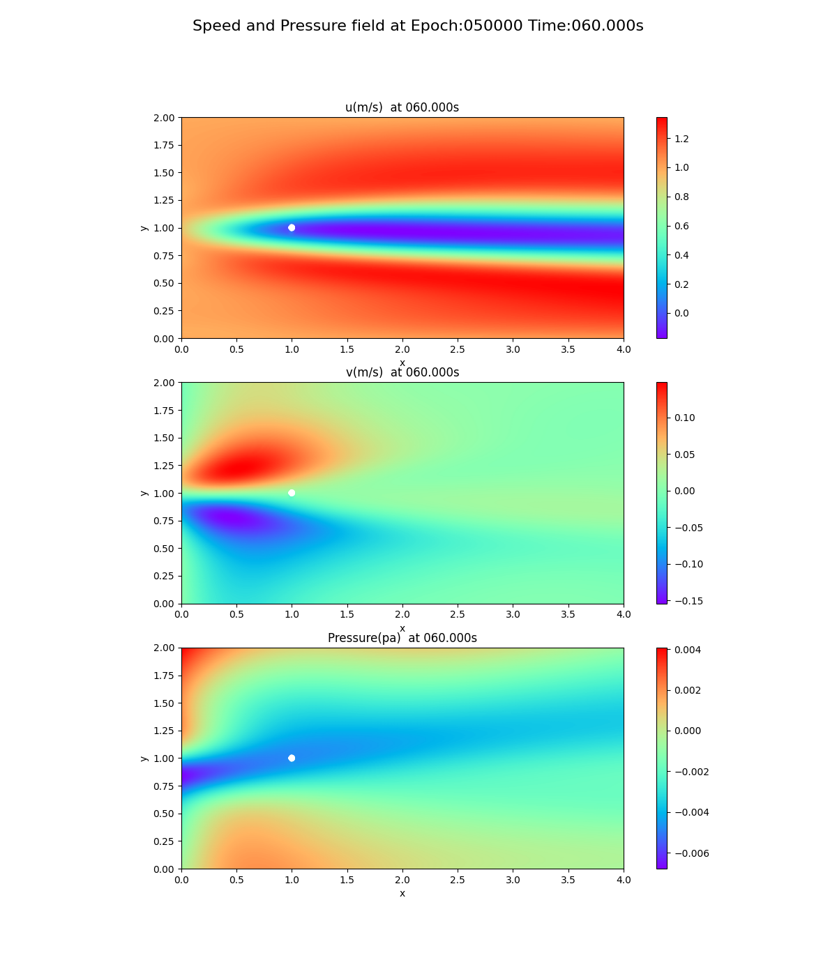
As can be seen from the loss curves, the loss seemed to converge after 20,000 cycles, so the results of training at 20,000 and 50,000 cycles are shown below. This is a snapshot at the end of the simulation (after 60 seconds).

20,000 epoch

uvp20K

50,000 epoch

uvp50K

Notice the pressure field. The slope (gradient) of the pressure field approaches 0 toward the x-axis direction, but this trend is not seen at 20,000 and 50,000 epoch.

Summary

The reason I chose 2D flow over a cylinder as my assignment was to see a Kalman vortex (vortex shedding) behind the cylinder, However, I learned that vortices are not possible with PINNs, as described in Kalman vortex with OpenFOAM. If so, I was going to build a simulation environment (code) with PINNs, even though vortices are not possible, in order to investigate and follow up on future research in the world.

The issue with my simulation results is that the nose in front of the cylinder (INLET direction) can be created compared to the flow prior in time to the vortex generation in OpenFoam. This was not improved by increasing the number of hidden layers, a trend that indicated convergence difficulties.

It was also found that even though the error curve appeared to converge, the pressure field required a large increase in the number of epochs before showing the expected results.

Perplexity and notebookLM were very useful in researching various related information on the Internet, with Perplexity playing the role of a scout who accesses papers on the Internet, and notebookLM playing the role of a staff member who learns the outline of the contents of the paper and then examines the details of the paper. I think that notebookLM has reduced the time to understand the content of English papers by an order of magnitude or more.