はじめに
深層学習day3の「Section1:再帰型ニューラルネットワークの概念」の実装演習を以下にまとめる。
実装演習
「3_1_simple_RNN.ipynb」を試した。
# 自分の環境で、ダウンロードした共通関数の格納フォルダのパス
import sys
sys.path.append('DNN_code_colab_lesson_3_4')
import numpy as np
from common import functions
import matplotlib.pyplot as plt
# def d_tanh(x):
def d_tanh(x):
return 1 / (np.cosh(x) ** 2)
# データを用意
# 2進数の桁数
binary_dim = 8
# 最大値 + 1
largest_number = pow(2, binary_dim)
# largest_numberまで2進数を用意
binary = np.unpackbits(np.array([range(largest_number)],dtype=np.uint8).T,axis=1)
input_layer_size = 2
hidden_layer_size = 16
output_layer_size = 1
weight_init_std = 1
learning_rate = 0.1
iters_num = 10000
plot_interval = 100
# ウェイト初期化 (バイアスは簡単のため省略)
W_in = weight_init_std * np.random.randn(input_layer_size, hidden_layer_size)
W_out = weight_init_std * np.random.randn(hidden_layer_size, output_layer_size)
W = weight_init_std * np.random.randn(hidden_layer_size, hidden_layer_size)
# Xavier
# He
# 勾配
W_in_grad = np.zeros_like(W_in)
W_out_grad = np.zeros_like(W_out)
W_grad = np.zeros_like(W)
u = np.zeros((hidden_layer_size, binary_dim + 1))
z = np.zeros((hidden_layer_size, binary_dim + 1))
y = np.zeros((output_layer_size, binary_dim))
delta_out = np.zeros((output_layer_size, binary_dim))
delta = np.zeros((hidden_layer_size, binary_dim + 1))
all_losses = []
for i in range(iters_num):
# A, B初期化 (a + b = d)
a_int = np.random.randint(largest_number/2)
a_bin = binary[a_int] # binary encoding
b_int = np.random.randint(largest_number/2)
b_bin = binary[b_int] # binary encoding
# 正解データ
d_int = a_int + b_int
d_bin = binary[d_int]
# 出力バイナリ
out_bin = np.zeros_like(d_bin)
# 時系列全体の誤差
all_loss = 0
# 時系列ループ
for t in range(binary_dim):
# 入力値
X = np.array([a_bin[ - t - 1], b_bin[ - t - 1]]).reshape(1, -1)
# 時刻tにおける正解データ
dd = np.array([d_bin[binary_dim - t - 1]])
u[:,t+1] = np.dot(X, W_in) + np.dot(z[:,t].reshape(1, -1), W)
z[:,t+1] = functions.sigmoid(u[:,t+1])
y[:,t] = functions.sigmoid(np.dot(z[:,t+1].reshape(1, -1), W_out))
#誤差
loss = functions.mean_squared_error(dd, y[:,t])
delta_out[:,t] = functions.d_mean_squared_error(dd, y[:,t]) * functions.d_sigmoid(y[:,t])
all_loss += loss
out_bin[binary_dim - t - 1] = np.round(y[:,t])
for t in range(binary_dim)[::-1]:
X = np.array([a_bin[-t-1],b_bin[-t-1]]).reshape(1, -1)
delta[:,t] = (np.dot(delta[:,t+1].T, W.T) + np.dot(delta_out[:,t].T, W_out.T)) * functions.d_sigmoid(u[:,t+1])
# 勾配更新
W_out_grad += np.dot(z[:,t+1].reshape(-1,1), delta_out[:,t].reshape(-1,1))
W_grad += np.dot(z[:,t].reshape(-1,1), delta[:,t].reshape(1,-1))
W_in_grad += np.dot(X.T, delta[:,t].reshape(1,-1))
# 勾配適用
W_in -= learning_rate * W_in_grad
W_out -= learning_rate * W_out_grad
W -= learning_rate * W_grad
W_in_grad *= 0
W_out_grad *= 0
W_grad *= 0
if(i % plot_interval == 0):
all_losses.append(all_loss)
print("iters:" + str(i))
print("Loss:" + str(all_loss))
print("Pred:" + str(out_bin))
print("True:" + str(d_bin))
out_int = 0
for index,x in enumerate(reversed(out_bin)):
out_int += x * pow(2, index)
print(str(a_int) + " + " + str(b_int) + " = " + str(out_int))
print("------------")
lists = range(0, iters_num, plot_interval)
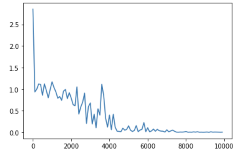
plt.plot(lists, all_losses, label="loss")
plt.show()
実行結果のグラフは次の通り。
「weight_init_std」を0.1、0.2、0.5、1.5、2と変化させた時の実行結果のグラフを以下に示す。
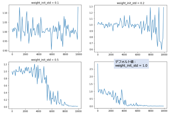
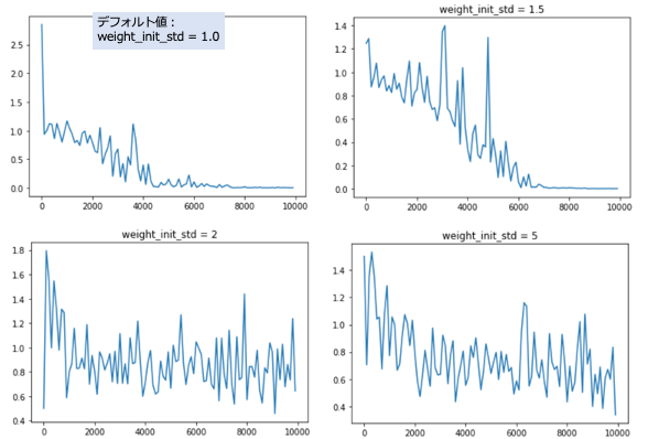
「weight_init_std」の値は、オリジナルの1が最も良い結果を示す。
0.5以下、1.5以上だと、学習が収束しないようだ。